With the release of the game Settlers of Catan in 1995, German inventor Klaus Teuber unleashed a product popular enough to introduce Americans to the Eurogame style of tabletop gaming. Per the Wikipedia entry, “A Eurogame, also called German-style board game, German game, or Euro-style game, is any of a class of tabletop games that generally have simple rules, short to medium playing times, indirect player interaction and abstract physical components. Such games emphasize strategy, downplay luck and conflict, lean towards economic rather than military themes, and usually keep all the players in the game until it ends.” The entry also describes how this class of games is contrasted with those referred to as “Ameritrash.” Interestingly, I read recently that the tradition of playing family games and board games was brought to America largely by German immigrants in the first place.
I was introduced to Settlers in about 2005 and have grown to appreciate more and more of the genre since. I particularly enjoy modular games as I’ve mentioned previously, but many of this class of strategy games are highly enjoyable. The thing that most interest me about them is that most games offer multiple ways to win. They usually involve a common end goal, like amassing a certain number of victory points, but there are generally different options for getting them. The strategy you adopt is based on how things evolve over the course of each game. This ensures that the games stay interesting a lot more often.
Many of us played Monopoly growing up, and it was a very popular game in America. The problem with Monopoly, however, is that there’s only one way to win. You have to grind you opponents into dirt, which can take a long time in some cases. My brother played in a Monopoly tournament at a local library when we were young, and he adopted a wheeler-dealer strategy that carried him to the finals and got him written up in the local paper. In the final game only one player was able to secure and develop a monopoly, and none of the other players would make trade to allow anyone else to do so. The game turned into something of a forced march that probably wasn’t that enjoyable. Monopoly was also interesting because it was one of the early games to be analyzed by computer, which recommended an optimum strategy based on the likelihood of landing on certain spaces. (Buy the orange properties.)

Some games of Monopoly kept everyone going over time until more and more money got injected into the game. Those games were always fun even if you didn’t win. A rather obscure stock market game called Bluechip had the same quality. Sometimes things were pretty thin and sometimes they were flush. If all players were flush then it could be a lot of fun. If all players were thin it was less fun but at least competitive. If some players were flush and others thin, and the difference could happen in your first turn, the fun level was cranked way down. I’ve heard Monopoly described as a one-mechanic game. There may be slightly more depending on how you define it but it is pretty straightforward. Bluechip was in every sense a one-dimensional game. I played it at a game convention a few years ago and saw it much differently than I had when I was younger. I saw that the strategy was very mechanical and without remorse. You simply made the biggest trade possible with the most leverage and hoped the cards and the dice didn’t work against you. Once I saw that the game got kind of stale. Oh well, at least I have the lovely memories of playing it with my grandparents!
One final note on Bluechip is that I’m almost certain it was the inspiration for a stock market simulation game called Millionaire, which was one of the first pieces of software released for the original Macintosh. It was apparently also available on some other platforms. We played it a lot at our house but the game is all but forgotten now. There aren’t even any references online good enough to link to.
The thing about Eurogames is that, in general, if the thing you were planning on isn’t working there may be a different avenue by which you can succeed. You always have to keep track of what everyone else is up to, balance your resources, defend, build, and often trade. In the basic edition of Settlers of Catan the object is to get ten victory points. You can do that by building settlements and upgrading them to cities, by building the longest road, or by buying development cards which give you the chance to earn victory points directly or build the largest army. The course you take depends on the resources you are able to acquire and the fall of the dice. The dice and the potential randomness of the board can skew the game away from one or more players but seldom is there a runaway by a single player. The game generally remains fun, engaging, and colorful for most participants, and it generally doesn’t take too long to play. Modular expansion kits and other versions of the game provide even more mechanics and possible trade-offs.
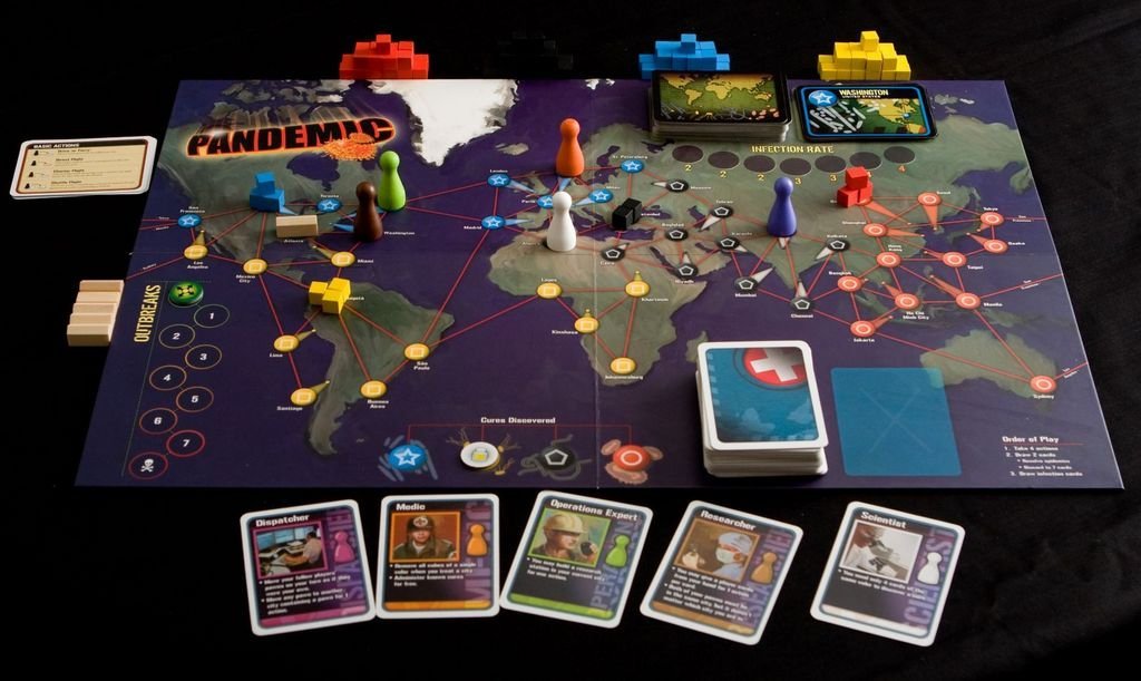
There is still another subclass of games in the Eurogame genre, and that is the cooperative game. In games like Pandemic the players all work together against a common enemy, which in this case is the worldwide spread of a virulently-communicable disease. Sometimes the players lose, but the players themselves are always on the same side.
I describe all this not because the games themselves are so thrilling, though I and many others certainly think they can be, but because they illustrate that there can be many ways to solve any possible problem. Boards games and certain competitions (e.g., American football and the buggy races held annually at my alma mater) provide specific contexts for those trade-offs. The art of balancing different factors in a specific context is known as a constrained optimization problem. The link is to a formalized mathematical approach to the subject but in many cases the constraints and possible solutions are explored by trial and error. A friend of mine from school told me that one of his professors observed that life, itself, is a constrained optimization problem.
I’m always interested in figuring out how to identify new twists on existing problems so certain classes of engineering and other problems always get my attention. I was taught early on to save on memory and execution time while writing software, but have since come to appreciate that development time, complexity, and maintainability are equally important considerations. I worked on a team that used analytical simulations to examine the effects of modifying different aspects of the logistics of maintaining and managing aircraft. I often have to balance the needs of customers and developers, the limits imposed by the iron triangle (cost, schedule, and scope in project management or software development), or the balance between work and life.
There are always real measurements, real constraints, real consequences, and real success and failure, but as I noted yesterday the goal is to approach every problem cooperatively when possible. The real world gives you enough win-lose and lose-lose propositions. Working together with others gives you the chance to develop solutions that are win-win. The more ways you can figure out to do that, the better.