
Having discussed the process of discovery yesterday I wanted to go into detail about data collection today. While discovery identifies the nouns and verbs of a process, data collection identifies the adjectives and adverbs. I’ve listed a bunch of ways to do both in this post on the observation technique, but here I’ll take a moment to describe how the collected data are used.
Data may be classified in several ways:
Continuous vs. Discrete: Continuous data can be represented numerically. This can include real numbers associated with physical dimensions, spans of time, amounts of energy, and intrinsic properties like hardness or pressure. This can also include counting variables that are usually integers, but not always. Discrete data items have to do with characteristics that aren’t necessarily numeric, like on or off, good or bad, colors, and so on. Interestingly, some of these can be represented numerically as discrete or continuous values. On/off is typically represented by one and zero (or boolean or logical), but color might be represented by names (e.g., blue or gray) or combinations of frequencies or brightness (like RGBA values).
Collected as point value or distribution: A point value is something that’s measured once and represents a single characteristic. A hammer might weight sixteen ounces and the interior volume of a mid-sized sedan might be 96.3 cubic feet. An example of distributed data would be a collection of times taken to complete an operation. Both continuous and discrete data can be calculated as distributions. A distribution of continuous data could be the weights of 237 beetles, while a distribution of discrete data could be the number of times an entity goes from one location to each of several possible new locations. A sufficient number of samples have to be collected for distributed data, which I discuss here.
Used as point value or distribution: Data collected as single point and distributed values can be used as point values. Single-to-single is straightforward but distributed-to-single is only a little more complicated. If a single point value is derived from a set of distributed values it will typically capture a single aspect of that collection. Examples are the average value, the mean, minimum, maximum, standard deviation, range, and a handful of others. Data used as distributed values must be collected from a distribution of data samples. There are a number of ways this can be done. Mostly this has to do with whether an interpolation will or will not be used to generate values between the sample data values.
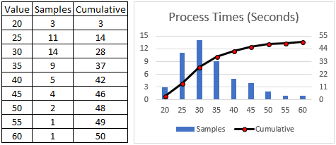
Given a two-column array based on the table above (in code we wouldn’t bother storing the values in the middle column), we’d generate a target value against the column of independent values, identify the “bucket” index, and then return the associated dependent value. In the case of the table above the leftmost column would be the dependent value and the rightmost column would be the independent value. This technique is good for discrete data like destinations, colors, or part IDs. If the target value was 23 (or 23.376) then the return value would be 30.
It’s also possible to interpolate between rows and generate outputs that weren’t part of the input data set.
The interesting thing about data used as a distribution is that only one resultant value is used at a time. There are two ways this could happen. One is to generate a point value for a one-time use (for example, the specific heat as a function of temperature for steel). The other is to generate a series of point values as part of a Monte Carlo analysis (for example, a continuous range of process times for some event). Monte Carlo results ultimately have to be characterized statistically.