R.P. Churchill.com | Adventures in Engineering and Life

Reproducing A Clever Animation Product, Part 2

Posted on June 1, 2016 by R.P. Churchill

Today I did some experiments to try to figure out why the animations I’ve created seem to hitch and hiccup slightly from time to time. Again, this work is based on recreating the basic functionality of the Greensock animation product described here and especially here.

The first thing I thought of was that the drawing operations themselves might be taking long enough that they don’t complete during every animation step (about 16 ms at 60 frames per second). I therefore set the update loop to only draw the items every other scan. This approach didn’t relieve the hitching and updating at 30 fps left the animation looking slightly choppy.

The next thing I tried was recording the elapsed time for every drawing loop and displaying the value if it was greater than 16 ms. However, the value was never displayed, so it appears that the speed of the drawing isn’t an issue.

Next it occurred to me that if an element has to travel far enough and in fine enough increments that the difference between traveling three or four pixels in an update, particularly when advancing by the smaller number doesn’t happen often, might be enough to look like a hitch. I therefore set the durations of the transitions to be shorter so each increment is larger, and I also incorporated a fade-in by ramping up the opacity. The combination of these two changes made things look pretty smooth.

I also observe that the example animation in the second Greensock link, above, involves transitions that are relatively short, so there isn’t time for anything to hitch. That may be the key to the whole enterprise. That said, there’s an animation in the first link that shows a fountain of green balls. I will try to reproduce something like that and see how it looks. Most of the effects can be replicated (though perhaps not as well as the originals), and I’ll be working through duplicating some of them over the next few posts.

In the meantime, I found it necessary to add an initialization capability so rerunning the animation starts from a good place. Here’s the basic code in its entirety.

<!DOCTYPE html>
<html>
  <head>
  	<title>Fast Animation Script Demo</title>
    <link type="text/css" rel="stylesheet" href="../stylesheet.css"/>

    <script type="text/javascript" src="jquery.min.js">
    </script>

    <style>
      .demo {
        height: 200px;
        width: 300px;
        margin-left: auto;
        margin-right: auto;
        background-color: #222222;
        display: block;
        overflow: hidden;
        position: relative;
      }
      .demoPanel {
        position: absolute;
        background-color: rgba(0,0,0,0);
        color: #EEEEEE;
        font-size: 1.2em;
      }
      #rerun_button {
        margin-left: auto;
        margin-right: auto;
        display: block;        
      }
    </style>
  </head>
  <body>
    <div class="demo">
      <div id="handle001" class="demoPanel"></div>
      <div id="handle002" class="demoPanel"></div>
    </div>
    <br />
    <button id="rerun_button" onclick="rerunClick()" style="height: 50px; width: 300px">Rerun the Animation</button>
    <br />
    <p id="elapsedElement"></p>
    <script>
      //specify element
      //specify initial properties
      //specify final properties
      //specify duration
      //specify start time
      //build list of commands that run for every animation call
      
      var bcActivitiesList = new Array;
      for (var i=0; i<1800; i++) {  //>
        bcActivitiesList[i] = new Array;
        bcActivitiesList[i][0] = 0;  //number of commands each animation step
      }  //30 seconds of activities
      var bcFinalActivity = -1;  //index of last animation activity
      
      var bcInitializations = new Array;
      bcInitializations[0] = 0;

      function bcInitElement(pElement,pLeft,pTop,pColor,pBackgroundColor,pWidth,pOpacity,pDisplay,innerHTML) {
        pElement.style.left = pLeft;
        pElement.style.top = pTop;
        pElement.style.color = pColor;
        pElement.style.backgroundColor = pBackgroundColor;
        pElement.style.width = pWidth;
        pElement.style.opacity = pOpacity;
        pElement.style.display = pDisplay;
        pElement.innerHTML = innerHTML;
      }
      function bcDefineLeftTween(sElement,pStart,pEnd,tBegin,tDuration,mMethod) {
        var s = sElement+".style.left='"+pStart+"px';"
        bcInitializations[0] = bcInitializations.push(s);
        var alpha = tBegin * 60.0;
        var steps = tDuration * 60;
        var omega = alpha + steps;
        var increment = (pEnd - pStart) / steps;
        var left = pStart;
        for (var i=alpha; i<=omega; i++) { //>
          s = sElement+".style.left='"+Math.round(left)+"px';"
          bcActivitiesList[i][0] = bcActivitiesList[i].push(s);
          if (mMethod == "linear") {
            left += increment;
          }
        }  
        if (omega > bcFinalActivity) {
          bcFinalActivity = omega;
        }
      }
      function bcDefineTopTween(sElement,pStart,pEnd,tBegin,tDuration,mMethod) {
        var s = sElement+".style.top='"+pStart+"px';"
        bcInitializations[0] = bcInitializations.push(s);
        var alpha = tBegin * 60.0;
        var steps = tDuration * 60;
        var omega = alpha + steps;
        var increment = (pEnd - pStart) / steps;
        var top = pStart;
        for (var i=alpha; i<=omega; i++) { //>
          s = sElement+".style.top='"+Math.round(top)+"px';"
          bcActivitiesList[i][0] = bcActivitiesList[i].push(s);
          if (mMethod == "linear") {
            top += increment;
          }
        }  
        if (omega > bcFinalActivity) {
          bcFinalActivity = omega;
        }
      }
      function bcDefineOpacityTween(sElement,pStart,pEnd,tBegin,tDuration,mMethod) {
        var s = sElement+".style.opacity='"+pStart+"';"
        bcInitializations[0] = bcInitializations.push(s);
        var alpha = tBegin * 60.0;
        var steps = tDuration * 60;
        var omega = alpha + steps;
        var increment = (pEnd - pStart) / steps;
        var opacity = pStart;
        for (var i=alpha; i<=omega; i++) { //>
          s = sElement+".style.opacity='"+opacity+"';"
          bcActivitiesList[i][0] = bcActivitiesList[i].push(s);
          if (mMethod == "linear") {
            opacity += increment;
          }
        }  
        if (omega > bcFinalActivity) {
          bcFinalActivity = omega;
        }
      }
      
      function bcInitializeElements() {
        var i = 1;
        while (i <= bcInitializations[0]) {  //>
          eval(bcInitializations[i]);
          i++;
        }
      }
      
      var elapsedHandle = document.getElementById("elapsedElement");
      function doSomeStuff(step) {
        var startTime = Date.now();
        var i = 1;
        while (i <= bcActivitiesList[step][0]) {  //>
          eval(bcActivitiesList[step][i]);
          i++;
        }
        var endTime = Date.now();
        var elapsed = endTime - startTime;
        if (elapsed > 16) {
          elapsedHandle.innerHTML = elapsed;
        } else {
          elapsedHandle.innerHTML = "";
        }
      } 
      
      var handle001 = document.getElementById("handle001");
      bcInitElement(handle001,"201px","50px","red","rgba(0,0,0,0)","260px",1,"block","This line slides in from the side");
      bcDefineLeftTween("handle001",301,25,0.0,0.75,"linear");
      bcDefineOpacityTween("handle001",0.0,1.0,0.0,0.75,"linear")
      
      var handle002 = document.getElementById("handle002");
      bcInitElement(handle002,"13px","-25px","blue","rgba(0,0,0,0)","280px",1,"block","This line drops down from the top");
      bcDefineTopTween("handle002",-25,125,0.5,0.75,"linear");
      bcDefineOpacityTween("handle002",0.0,1.0,0.5,0.75,"linear")
      
      var maxAnimationSteps = bcFinalActivity;

      bcInitializeElements();
      var animationStep = 0;
      var requestId;
      function animateSomeStuff() {
        doSomeStuff(animationStep);
        if (animationStep >= maxAnimationSteps) {
          cancelAnimationFrame(requestID);
        } else {
          animationStep++;
        } 
        requestId = window.requestAnimationFrame(animateSomeStuff);      
      }
      animateSomeStuff();
      
      function rerunClick() {  //called on button click
        animationStep = 0;
        bcInitializeElements();
        animateSomeStuff();
      }
      

    </script>
  </body>
</html>

100

101

102

103

104

105

106

107

108

109

110

111

112

113

114

115

116

117

118

119

120

121

122

123

124

125

126

127

128

129

130

131

132

133

134

135

136

137

138

139

140

141

142

143

144

145

146

147

148

149

150

151

152

153

154

155

156

157

158

159

160

161

162

163

164

165

166

167

168

169

170

171

172

173

174

175

176

177

178

179

180

181

182

183

184

185

186

187

188

189

<!DOCTYPE html>

<html>

<head>

<title>Fast Animation Script Demo</title>

</script>

<style>

.demo {

height: 200px;

width: 300px;

margin-left: auto;

margin-right: auto;

background-color: #222222;

display: block;

overflow: hidden;

position: relative;

}

.demoPanel {

position: absolute;

background-color: rgba(0,0,0,0);

color: #EEEEEE;

font-size: 1.2em;

}

#rerun_button {

margin-left: auto;

margin-right: auto;

display: block;

}

</style>

</head>

<body>

</div>

<br />

<button id="rerun_button" onclick="rerunClick()" style="height: 50px; width: 300px">Rerun the Animation</button>

<br />

//specify element

//specify initial properties

//specify final properties

//specify duration

//specify start time

//build list of commands that run for every animation call

var bcActivitiesList = new Array;

for (var i=0; i<1800; i++) { //>

bcActivitiesList[i] = new Array;

bcActivitiesList[i][0] = 0; //number of commands each animation step

} //30 seconds of activities

var bcFinalActivity = -1; //index of last animation activity

var bcInitializations = new Array;

bcInitializations[0] = 0;

function bcInitElement(pElement,pLeft,pTop,pColor,pBackgroundColor,pWidth,pOpacity,pDisplay,innerHTML) {

pElement.style.left = pLeft;

pElement.style.top = pTop;

pElement.style.color = pColor;

pElement.style.backgroundColor = pBackgroundColor;

pElement.style.width = pWidth;

pElement.style.opacity = pOpacity;

pElement.style.display = pDisplay;

pElement.innerHTML = innerHTML;

}

function bcDefineLeftTween(sElement,pStart,pEnd,tBegin,tDuration,mMethod) {

var s = sElement+".style.left='"+pStart+"px';"

bcInitializations[0] = bcInitializations.push(s);

var alpha = tBegin * 60.0;

var steps = tDuration * 60;

var omega = alpha + steps;

var increment = (pEnd - pStart) / steps;

var left = pStart;

for (var i=alpha; i<=omega; i++) { //>

s = sElement+".style.left='"+Math.round(left)+"px';"

bcActivitiesList[i][0] = bcActivitiesList[i].push(s);

if (mMethod == "linear") {

left += increment;

}

if (omega > bcFinalActivity) {

bcFinalActivity = omega;

}

function bcDefineTopTween(sElement,pStart,pEnd,tBegin,tDuration,mMethod) {

var s = sElement+".style.top='"+pStart+"px';"

bcInitializations[0] = bcInitializations.push(s);

var alpha = tBegin * 60.0;

var steps = tDuration * 60;

var omega = alpha + steps;

var increment = (pEnd - pStart) / steps;

var top = pStart;

for (var i=alpha; i<=omega; i++) { //>

s = sElement+".style.top='"+Math.round(top)+"px';"

bcActivitiesList[i][0] = bcActivitiesList[i].push(s);

if (mMethod == "linear") {

top += increment;

}

if (omega > bcFinalActivity) {

bcFinalActivity = omega;

}

function bcDefineOpacityTween(sElement,pStart,pEnd,tBegin,tDuration,mMethod) {

var s = sElement+".style.opacity='"+pStart+"';"

bcInitializations[0] = bcInitializations.push(s);

var alpha = tBegin * 60.0;

var steps = tDuration * 60;

var omega = alpha + steps;

var increment = (pEnd - pStart) / steps;

var opacity = pStart;

for (var i=alpha; i<=omega; i++) { //>

s = sElement+".style.opacity='"+opacity+"';"

bcActivitiesList[i][0] = bcActivitiesList[i].push(s);

if (mMethod == "linear") {

opacity += increment;

}

if (omega > bcFinalActivity) {

bcFinalActivity = omega;

}

function bcInitializeElements() {

var i = 1;

while (i <= bcInitializations[0]) { //>

eval(bcInitializations[i]);

i++;

}

var elapsedHandle = document.getElementById("elapsedElement");

function doSomeStuff(step) {

var startTime = Date.now();

var i = 1;

while (i <= bcActivitiesList[step][0]) { //>

eval(bcActivitiesList[step][i]);

i++;

}

var endTime = Date.now();

var elapsed = endTime - startTime;

if (elapsed > 16) {

elapsedHandle.innerHTML = elapsed;

} else {

elapsedHandle.innerHTML = "";

}

var handle001 = document.getElementById("handle001");

bcInitElement(handle001,"201px","50px","red","rgba(0,0,0,0)","260px",1,"block","This line slides in from the side");

bcDefineLeftTween("handle001",301,25,0.0,0.75,"linear");

bcDefineOpacityTween("handle001",0.0,1.0,0.0,0.75,"linear")

var handle002 = document.getElementById("handle002");

bcInitElement(handle002,"13px","-25px","blue","rgba(0,0,0,0)","280px",1,"block","This line drops down from the top");

bcDefineTopTween("handle002",-25,125,0.5,0.75,"linear");

bcDefineOpacityTween("handle002",0.0,1.0,0.5,0.75,"linear")

var maxAnimationSteps = bcFinalActivity;

bcInitializeElements();

var animationStep = 0;

var requestId;

function animateSomeStuff() {

doSomeStuff(animationStep);

if (animationStep >= maxAnimationSteps) {

cancelAnimationFrame(requestID);

} else {

animationStep++;

}

requestId = window.requestAnimationFrame(animateSomeStuff);

}

animateSomeStuff();

function rerunClick() { //called on button click

animationStep = 0;

bcInitializeElements();

animateSomeStuff();

}

</script>

</body>

</html>

Reproducing A Clever Animation Product, Part 1

Posted on May 31, 2016 by R.P. Churchill

I’ve been working on an introductory animation for my soon-to-be-released landing page (what, stumbling into a random WordPress post and a tiny resume link isn’t the pithiest possible introduction?), and I was looking around and playing with various ideas when I stumbled across this site and this video. This company makes what look to be a very impressive set of products with even more impressive licensing terms. However, since the point of this website, for now, is to help me learn new things when I’m not describing and recreating some of the work I’ve done from earlier in my career, I used the information presented as inspiration for creating my own basic animation framework.

The first thing I want to point out as I begin this week of related posts is that I haven’t looked at the company’s and product’s code at all. I’m just trying to recreate some basic functionality and use what I see as inspiration for my own explorations. The things I found helpful were the ideas embodied in the animation product. I would not assume that I’ve figured out exactly how they did what they did but I’ve definitely been able to recreate some of the same functionality in my own way. This is in keeping with my goal of ensuring that all the running code on this site is my own.

If you check out the linked video you see a tool that uses a very terse JavaScript syntax that produces very nice, very controllable effects. The key thing is that the animations produced run quickly and smoothly. I a) needed an animation and b) like to build tools so this was a natural thing to tackle.

I spent some of the past weekend building up a rather cumbersome first attempt at an animation framework. It was big and it was kludgy and it was slow and it sometimes hiccuped. I recognized that I needed a system that carried out the following steps:

specify element
specify initial properties
specify final properties
specify duration
specify start time
build list of commands that run for every animation call

What I originally came up with was a way to create an array with links bunch of elements, create arrays with transformation objects that describe what to do with each element, and a way to cycle through the lists of elements and transformations to see what needs to be done… during every animation step. Since the animation steps might be happening every 60th of a second on a modern device (possibly less often on an older machine… like a Palm Pre like maybe), you can imagine there’s quite a bit of overhead. I also made the original animation space rather large which involved long traversals that took up a decent amount of time. The original animations worked but they took a lot of code to express and like I said, they weren’t always very smooth. Then I noticed a couple of things that helped.

One was that the example animation shown in the linked video was comparatively small, and the transitions all happened rather quickly. I therefore resolved to make my intro animation much smaller. I chose a 400-by-400 pixel space for the animation, which fits my page and should look respectable on any modern device. I don’t promise that any example I develop during these experiments will run well (or even at all) on every device, in every browser, and on every OS, but it should work and look reasonable on anything current. I’m also assuming a 60 frames-per-second refresh rate. I’ll explain why tomorrow.

The other thing I noticed is that the verbiage on the company’s site spoke of creating tweens for each animation step. This suggested that the product wasn’t figuring out what to do during every animation step, but was probably pre-calculating the actions up front. I ended up rewriting something that was much, much more succinct in terms of code and ran a heck of a lot more smoothly.

It takes a certain amount of information to describe the actions to be taken, and the incredibly terse JavaScript that does so in the linked video seems to leave some of it out. Or, rather, it makes certain assumptions about where things begin and end. I created a function that linked to elements in the animation div (I made them all divs themselves but they could be anything and it would probably be more efficient if most of them weren’t divs) and another set of functions that calculate tweens and load them into a list of commands to be executed as the animation proceeds. It occurred to me that the JavaScript files written by the company probably do something similar, and the impossibly pithy code the users write is actually something that gets peeled apart, interpreted, and fed to a series of functions similar to what I wrote. I don’t know that to be true, I just feel like it might be.

The thing that ultimately makes the thing go, and go smoothly, is the list of commands to be processed during each animation step. Remember from a recent post that the basic animation loop works something like this:

    var maxAnimationSteps = ...;

    function doSomeStuff(step) {...}

    var animationStep = 0;
    var requestId;
    function animateSomeStuff() {
      doSomeStuff(animationStep);
      if (animationStep >= maxAnimationSteps {
        cancelAnimationFrame(requestId);
      } else {
        animationStep++;
      }
      requestId = window.requestAnimationFrame(animateSomeStuff);      
    }
    animateSomeStuff();

var maxAnimationSteps = ...;

function doSomeStuff(step) {...}

var animationStep = 0;

var requestId;

function animateSomeStuff() {

doSomeStuff(animationStep);

if (animationStep >= maxAnimationSteps {

cancelAnimationFrame(requestId);

} else {

animationStep++;

}

requestId = window.requestAnimationFrame(animateSomeStuff);

}

animateSomeStuff();

What you want, therefore, is the pithiest possible set of commands to run in the doSomeStuff call. I use the animationStep variable as an index into the array of animation commands I set up prior to kicking off the animation loop. The array of animation commands has two dimensions, one for each animation step, and one for each command issued during that step. (I happened to reserve element zero in each secondary array for holding the number of commands to be issued but that isn’t strictly necessary.) When the animation runs for each time step all it has to do is cycle through the list of activities that has to be performed during that animation step.

So, how do you–pithily–tell the program how to manipulate some aspect of an HTML element? Wouldn’t it be nice if we had access to something simple like:

  document.getElementById("nameOfItem").style.cssProperty = value;

1	document.getElementById("nameOfItem").style.cssProperty = value;

…where we could refer to a known JavaScript handle, a specific property, and a specific value? Well, using the concept of automatic code generation it’s a simple matter to generate a bit of text like the following, which represents a valid line of JavaScript code that can be stored in the second dimension of the array of animation commands.

“handle001.style.left = ‘117px’;”

I also happened to be reading through some advice on JavaScript programming, which says to NOT use the eval() command, but this seemed almost too good to be true. If we feed the generated string to the eval command we can do just about anything. There may be some overhead from using this method, but it certainly gets the job done.

It is entirely possible that the good people at Greensock came up with a better way to do this, and I’m sure that there are, in fact, many ways to accomplish this sort of thing. This method does have the virtue of being compact and straightforward, and, most importantly, it more or less works.

I’ll go into more detail in subsequent posts but here is a very simple example of the process in action.

The red line slides in from the left over one second starting from time zero. The blue line drops down from the bottom over two seconds starting from the 0.5-second mark. All parameters are settable.

As I look at this I see that the process keeps hitching and hiccuping, so it’s very likely that I’m missing something. It’s possible that the eval() function is not the best way to do things, and it’s also possible that the problem lies elsewhere. The elements I’m moving are divs, which require more overhead to move than just raw HTML elements, and I’m also updating every element during every animation step (60 fps on modern devices). It’s possible that I can skip animation steps and still get decent effects.

Posted in Tools and methods | Tagged animation, fast animation framework, JavaScript | Leave a comment

Prettying Up the 3D Graph Output

Posted on May 26, 2016 by R.P. Churchill

Here I’ve prettied the graph up so the lines change color every 100 degrees F, and I’ve added a legend. I suppose I could choose consecutive colors with a bit more contrast.

Posted in Tools and methods | Tagged animation, canvas, matrix solution techniques, simulation, sim_presentation_series, thermodynamics | Leave a comment

Graphing the Matrix Output

Posted on May 25, 2016 by R.P. Churchill

Here I continually run the heating routine for a piece with an initial temperature of 70 degrees in a furnace set to 2300 degrees. The temperature scale, expressed vertically, runs from 0-2500 degrees. The bottom of the piece, which sits on a solid hearth through which no heat is transferred, is to the lower right.

The graph is rendered using a shortcut isometric technique which obviates the need for matrix multiplications and perspective transformations.

Posted in Tools and methods | Tagged animation, canvas, matrix solution techniques, simulation, sim_presentation_series, thermodynamics | Leave a comment

How Quickly Can the Matrix Be Solved On Different Machines?

Posted on May 24, 2016 by R.P. Churchill

Today I ran 2750 iterations of the matrix on some additional machines.

My 64GB iPad 3 runs a 1 GHz, dual-core, 32-bit, ARM Cortex-A9 and ran the test in 1.308 seconds on load and about 1.15 seconds on rerun.

My MacBook Pro from 2013 runs a 2.7 GHz Core i7 and did the initial run in 0.09-0.130 seconds and re-runs in as little as 0.070 seconds. That’s almost as fast as my 2015 notebook PC.

I wasn’t kidding about digging up my old Palm Pre, either. I finally got it charged up and running but found it would only run up to 500 iterations before it would hang. I therefore created another version of the test which runs only 500 iterations, as shown below.

The Pre Plus, a 500 MHz ARM Cortex-A8, managed to grind through 500 iterations in 4.77 seconds. At that rate it would take 25.85 seconds to do 2750 iterations. That is slower than what a good desktop machine from the late 1990s could do. A couple of thoughts occur to me, however. The Palm Pre was introduced to great fanfare but had numerous problems from the beginning. What was left of Palm didn’t have the resources to get the software into the best shape when it was released (the ability to record video was only enabled after a handful of OS updates). I would not be surprised if the code for the browser or JavaScript implementation were less than optimal. The company was acquired by HP, which then managed to drive the final nails into Palm’s coffin.

Still, the matrix code doesn’t make use of any special or new features of HTML, CSS, or JavaScript and did manage to run to completion, so I guess that’s an interesting finding on its own. It’s kind of like the poodles in tutus that used to walk on their hind legs on the old Ed Sullivan Show. You weren’t impressed that they did it well, what was impressive is that they could do it at all.

Posted in Tools and methods | Tagged changing technology, efficiency, JavaScript, matrix solution techniques, sim_presentation_series | Leave a comment

How Quickly Can the Matrix Be Solved?

Posted on May 23, 2016 by R.P. Churchill

The solution was finally made to run last week. Today the question is how fast the thing runs. My feel for the answer to this question has to do with the context in which I first asked it.

From 1994 to 2000 the fastest desktop computers I worked with maxed out at 400 MHz. That was true for PCs and the more expensive DEC Vax and Alpha machines we were running. By contrast the laptop I’m working on uses an Intel Core i7-4510U CPU with a base speed of 2.00 GHz. That would be five times faster on its own. However, that number is the base speed of each core, and depending on the number running the speed can theoretically be boosted to as much as 3.1 GHz. The Windows system page indicates that the fastest core may be running at 2.6 GHz.

After that we can consider that each core in a current CPU is likely to be further optimized in terms of its internal architecture, the number of clock cycles it takes to perform each operation, the amount of available cache memory, the speed at which data can be moved in and out of RAM, and other considerations. The current chip and OS is also 64 bits while the older ones were only 32 bits, though that consideration may not have much effect on the speed of calculations.

I don’t know how to evaluate the overhead incurred by the operating system itself, but running JavaScript in a browser at least carries the overhead of the browser.

Next we can consider the number of times the matrix code had to be run for every model iteration. The matrix had to be run at least once to update the current temperature of each piece in the furnace during each time step. The number of pieces in a furnace could range from, say, 8 to 144 depending on the application, so lets pick 50 for giggles. This number doesn’t really matter because the bulk of the work is done when trying to predict what happens in the future.

Control systems based on model-predictive simulation work by starting from current conditions and calculating what will happen in the future. If the results obtained by the simulation match the desired results then the control settings need not be changed. However, if the predicted results do not match the desired results the program has to figure out what control inputs to change. Without going into detail, the furnace Level 2 systems I wrote would march the pieces out of the furnace at the current average pace of movement through the furnace, figure out what the discharge average and differential temperatures (the difference between the temperatures of the hottest and coldest nodes in a particular piece, which value had to be below a specified threshold) would be, compare the predicted result with the desired result, and adjust the control settings.

The control settings adjusted by the Level 2 system were the temperature setpoints for each zone in the furnace. A furnace might have anywhere from one to six (or more) independently controlled zones. It was up to the Level 1 systems to do the detailed work necessary to make this happen. They used PLCs to control gas flows, fuel-air ratios, pressures, movements, cooling, opening and closing of doors, operation of exhaust flues, safety systems, and so on. They were a whole world of their own and I was always thoroughly impressed with the people who built those systems.

For this example I’ve assumed that there are three effective zones of control in the furnace, and the predicted temperature of at least one piece has to be calculated for each zone. The “critical” piece in each zone was the one that was logically identified to be the hardest to heat. Pieces could be a bit over temperature of more thoroughly soaked (lower than target differential temperature, but if they were too cold or not sufficiently soaked they could break a mill stand, which would slow the operation down). As the pieces are being marched out of the furnace the prediction code assumes that the Level 1 system will move the furnace temperatures to their setpoints for each zone if they are not already there. I ran successive iterations of the prediction code until I either got the discharge temperatures to within a few degrees of their targets or until the number of iterations gets up to five. Greater accuracy could be achieved during later time steps but the model could never be allowed to run longer than its designated time step.

Next I considered the pace of movement through the furnace. If the furnace was running slowly it might take two hours for a piece to get through the furnace, and that would mean 180 40-seecond time steps. So, at 3 pieces times 5 iterations times 180 steps we have 2700 matrix calculations. More are certainly possible.

I’ve set the example up to run 2750 iterations, which would be enough to update 50 pieces plus predict three as described. The code runs when the page is first loaded and again whenever the button is clicked. I noticed that clicking the button to repeat the test yields notably better results, so there must be some overhead associated with the initial load of the page.

I would have expected the code to take 5-10 seconds to run, but on my laptop, with the file served from local disk, the initial result was 0.08 seconds and about 0.05 when the button is clicked to rerun. This represents a performance improvement of at least 100, which is kind of mind-blowing to me.

Served over a fast connection from the website I get results of about 0.085 seconds on load and 0.052 seconds on rerun.

On my iPhone 5S I get 0.352 seconds on load and 0.230 seconds on rerun. That may be even more mind-blowing.

Tomorrow I’ll try this on a few other systems to see how it feels. What results are you getting on your setup?

Posted in Tools and methods | Tagged changing technology, efficiency, JavaScript, matrix solution techniques, model-predictive control, simulation, sim_presentation_series | Leave a comment

Finally Solving the Matrix

Posted on May 19, 2016 by R.P. Churchill

Once we get all the parameters calculated and the matrix loaded, then we can finally solve the thing. Here’s how the code looks:

    function loadMatrix(index,fceTemp)
    {
      var i; var j; var k;
      var tsa; var tfa; var ts3; var tf4;

      tfa = arrayTfce[index] + Tabs;
      tf4 = tfa * tfa * tfa * tfa;

      for (k = 0; k <= sizeNodes; k++)
      {
        ZSRCE[k] = 0.0;
        ZAUX[k] = 0.0;
        for (i = 0; i <= sizeBandWidth; i++)
          ZMATX[k][i] = 0.0;
      }

      k = 0;
      for (j = 0; j < nodesHigh; j++)
        for (i = 0; i < nodesWide; i++)
        {
          k++;

          //nodal energy
          ZMATX[k][1] += arrayRho[i][j] * arrayCp[i][j];
          ZSRCE[k] += arrayRho[i][j] * arrayCp[i][j] * arrayT[i][j];

          //conduction to right
          if (arrayKright[i][j] > 0.0)
          {
            ZMATX[k][1] += arrayKright[i][j];
            ZMATX[k][2] -= arrayKright[i][j];
            ZMATX[k+1][1] += arrayKright[i][j];
          }

          //conduction up
          if (arrayKup[i][j] > 0.0)
          {
            ZMATX[k][1] += arrayKup[i][j];
            ZMATX[k][1+nodesWide] -= arrayKup[i][j];
            ZMATX[k+nodesWide][1] += arrayKup[i][j];
          }

          //radiation
          if (arrayRad[i][j] > 0.0)
          {
            tsa = arrayT[i][j];
            ts3 = tsa * tsa * tsa;
            ZMATX[k][1] += arrayRad[i][j] * ts3;
            ZSRCE[k] += arrayRad[i][j] * tf4;
          }

        }
    }     //loadMatrix

    function oneCalc(index) {
      calcParams(index);

      for (var i=0; i<nodesWide; i++) {
        for (var j=0; j<nodesHigh; j++) {
          arrayT[i][j] = arrayTpieces[index][i][j] + Tabs;
        }
      }
      
      loadMatrix(index);
      calcMatrix();
      
      k = 0;
      for (var j=0; j<nodesHigh; j++) {
        for (var i=0; i<nodesWide; i++) {
          k++;
          arrayTpieces[index][i][j] = ZSRCE[k] - Tabs;
        }
      }
    }  //oneCalc

    var loopCount = 0;
    
    var s="Temperatures after "+loopCount+" time steps<br />";
    for (var j=nodesHigh-1; j>=0; j--) {
      for (var i=0; i<=nodesWide-1; i++) {
        s += arrayTpieces[0][i][j].toPrecision(7) + ", ";
      }
      s += "<br />";
    }
    document.getElementById("stuff").innerHTML = s;

    function runOneTime() {
      if (loopCount == 0) {
        for (var i=0; i< pieceCount; i++) {
          for (var j=0; j<nodesWide; j++) {
            for (var k=0; k<nodesHigh; k++) {
              arrayTpieces[i][j][k] = 70.0;
            }
          }
        }
      } else {
        oneCalc(0);
      }
      var s="Temperatures after "+loopCount+" time steps<br />";
      for (var j=nodesHigh-1; j>=0; j--) {
        for (var i=0; i<=nodesWide-1; i++) {
          s += arrayTpieces[0][i][j].toPrecision(7) + ", ";
        }
        s += "<br />";
      }
      document.getElementById("stuff").innerHTML = s;
      loopCount++;
      if (loopCount > 20) {
        loopCount = 0;
      }
    }

    var intervalID = setInterval(runOneTime, 1000);

100

101

102

103

104

105

106

107

108

109

110

111

112

113

function loadMatrix(index,fceTemp)

{

var i; var j; var k;

var tsa; var tfa; var ts3; var tf4;

tfa = arrayTfce[index] + Tabs;

tf4 = tfa * tfa * tfa * tfa;

for (k = 0; k <= sizeNodes; k++)

{

ZSRCE[k] = 0.0;

ZAUX[k] = 0.0;

for (i = 0; i <= sizeBandWidth; i++)

ZMATX[k][i] = 0.0;

}

k = 0;

for (j = 0; j < nodesHigh; j++)

for (i = 0; i < nodesWide; i++)

{

k++;

//nodal energy

ZMATX[k][1] += arrayRho[i][j] * arrayCp[i][j];

ZSRCE[k] += arrayRho[i][j] * arrayCp[i][j] * arrayT[i][j];

//conduction to right

if (arrayKright[i][j] > 0.0)

{

ZMATX[k][1] += arrayKright[i][j];

ZMATX[k][2] -= arrayKright[i][j];

ZMATX[k+1][1] += arrayKright[i][j];

}

//conduction up

if (arrayKup[i][j] > 0.0)

{

ZMATX[k][1] += arrayKup[i][j];

ZMATX[k][1+nodesWide] -= arrayKup[i][j];

ZMATX[k+nodesWide][1] += arrayKup[i][j];

}

//radiation

if (arrayRad[i][j] > 0.0)

{

tsa = arrayT[i][j];

ts3 = tsa * tsa * tsa;

ZMATX[k][1] += arrayRad[i][j] * ts3;

ZSRCE[k] += arrayRad[i][j] * tf4;

}

} //loadMatrix

function oneCalc(index) {

calcParams(index);

for (var i=0; i<nodesWide; i++) {

for (var j=0; j<nodesHigh; j++) {

arrayT[i][j] = arrayTpieces[index][i][j] + Tabs;

}

loadMatrix(index);

calcMatrix();

k = 0;

for (var j=0; j<nodesHigh; j++) {

for (var i=0; i<nodesWide; i++) {

k++;

arrayTpieces[index][i][j] = ZSRCE[k] - Tabs;

}

} //oneCalc

var loopCount = 0;

var s="Temperatures after "+loopCount+" time steps<br />";

for (var j=nodesHigh-1; j>=0; j--) {

for (var i=0; i<=nodesWide-1; i++) {

s += arrayTpieces[0][i][j].toPrecision(7) + ", ";

}

s += "<br />";

}

document.getElementById("stuff").innerHTML = s;

function runOneTime() {

if (loopCount == 0) {

for (var i=0; i< pieceCount; i++) {

for (var j=0; j<nodesWide; j++) {

for (var k=0; k<nodesHigh; k++) {

arrayTpieces[i][j][k] = 70.0;

}

} else {

oneCalc(0);

}

var s="Temperatures after "+loopCount+" time steps<br />";

for (var j=nodesHigh-1; j>=0; j--) {

for (var i=0; i<=nodesWide-1; i++) {

s += arrayTpieces[0][i][j].toPrecision(7) + ", ";

}

s += "<br />";

}

document.getElementById("stuff").innerHTML = s;

loopCount++;

if (loopCount > 20) {

loopCount = 0;

}

var intervalID = setInterval(runOneTime, 1000);

We start with a 7×7-node workpiece where the interior nodes are two inches wide and two inches high. The surface nodes are half as wide or high, meaning the cross-section area of each node is four square inches in the interior of the piece, one square inch on the four corners of the piece, and two square inches for the other surface nodes. The length of the surface exposed to the furnace is zero for interior nodes, zero for the bottom middle nodes (the piece is sitting on a solid hearth through which it is assumed no heat transfer occurs), one inch for the bottom nodes on each side, and two inches for the remaining surface nodes (the two corner nodes include one inch across the top surface and one inch down the side surface). The center of each interior node is assumed to be in the middle of the node, one inch from each side. The “center” of each surface node is assumed to be on the middle of the outer surface of the node. The “center” of the outer corner nodes is assumed to be on the outermost corner. This way there are always exactly two inches between the centers of each node, so the heat conduction terms make sense and the radiation can “see” the “center” of each node.

I have done it this way from the beginning and found that the readings of surface temperature on pieces which were actually heated in furnace matched the predicted values with impressive accuracy.

If all nodes are initialized to 70 degrees F, then exposed to a furnace at 1800 degrees F for successive 40-second time steps, we get the following results:

Posted in Tools and methods | Tagged matrix solution techniques, sim_presentation_series, thermodynamics | Leave a comment

Dimensions and Other Considerations Before We Solve the Matrix

Posted on May 18, 2016 by R.P. Churchill

Yesterday’s post showed how some of the constants and parameters are initialized or calculated. Today we’ll describe a few more.

This exercise defines a cross-section of a steel billet that is 8 inches by 8 inches and divided into five nodes high and five nodes wide. I found it convenient to assume the surface nodes were only half the height or width of the middle nodes, and to assume the center of surface nodes is on the outer edge or corner of the node, or in the middle of the node for central nodes. This means that the centers are always equidistant both across and up. The surface nodes also receive conducted heat and radiated heat at the same location. Nodes on the corners have one quarter the cross-sectional area of the fully central nodes, and nodes on the surface but not on the corner have one half the area of the fully central nodes.

    var timeStep = 40.0;  //seconds
    
    var nodeWidth = 2.0;   //inches
    var nodeHeight = 2.0;  //inches
    
    var pieceCount = 50;
    
    var arrayTpieces = new Array;
    var arrayT = new Array;
    for (var i=0; i< pieceCount; i++) {
      arrayTpieces[i] = new Array;
      for (var j=0; j<nodesWide; j++) {
        arrayTpieces[i][j] = new Array;
        arrayT[j] = new Array;
        for (var k=0; k<nodesHigh; k++) {
          arrayTpieces[i][j][k] = 70.0;
          arrayT[j][k] = 0.0;
        }
      }
    }
    var arrayTfce = new Array;
    for (var i=0; i< pieceCount; i++) {
      arrayTfce[i] = 1800.0;
    }      
    
    var arrayRho = new Array;
    var arrayCp = new Array;
    var arrayKup = new Array;
    var arrayKright = new Array;
    var arrayDup = new Array;
    var arrayDright = new Array;
    var arrayArea = new Array;
    var arraySurfLength = new Array;
    var arrayVF = new Array;
    var arrayRad = new Array;
    var tempLength = 0.0;
    for (var i=0; i<nodesWide; i++) {
      arrayRho[i] = new Array;
      arrayCp[i] = new Array;
      arrayKup[i] = new Array;
      arrayKright[i] = new Array;
      arrayDup[i] = new Array;
      arrayDright[i] = new Array;
      arrayArea[i] = new Array;
      arraySurfLength[i] = new Array;
      arrayVF[i] = new Array;
      arrayRad[i] = new Array;
      for (j=0; j<nodesHigh; j++) {
        arrayRho[i][j] = 0.0;
        arrayCp[i][j] = 0.0;
        arrayKup[i][j] = 0.0;
        arrayKright[i][j] = 0.0;
        if (j < nodesHigh-1) {  
          arrayDup[i][j] = nodeHeight;
        } else {  
          arrayDup[i][j] = 0.0;
        }
        if (i < nodesWide-1) {  
          arrayDright[i][j] = nodeWidth;
        } else {  
          arrayDright[i][j] = 0.0;
        }
        arrayArea[i][j] = nodeHeight * nodeWidth;
        if ((i == 0) || (i == nodesWide-1)) {
          arrayArea[i][j] *= 0.5;
        }
        if ((j == 0) || (j == nodesHigh-1)) {
          arrayArea[i][j] *= 0.5;
        }
        arraySurfLength[i][j] = 0.0;
        arrayVF[i][j] = 0.0;
        if (j == nodesHigh-1) {
          if ((i == 0) || (i == nodesWide-1)) {
            arraySurfLength[i][j] += nodeWidth * 0.5;
          } else {
            arraySurfLength[i][j] += nodeWidth;
          }
          arrayVF[i][j] = 1.0 * arraySurfLength[i][j];
        }
        tempLength = 0.0;
        if ((i == 0) || (i == nodesWide-1)) {
          if ((j == 0) || (j == nodesHigh-1)) {
            arraySurfLength[i][j] += nodeHeight * 0.5;
            tempLength = nodeHeight * 0.5;
          } else {
            arraySurfLength[i][j] += nodeHeight;
            tempLength = nodeHeight;
          }
          if (j == 0) {arrayVF[i][j] += 0.26 * tempLength;}
          else if (j == 1) {arrayVF[i][j] += 0.41 * tempLength;}
          else if (j == 2) {arrayVF[i][j] += 0.55 * tempLength;}
          else if (j == 3) {arrayVF[i][j] += 0.67 * tempLength;}
          else if (j == 4) {arrayVF[i][j] += 0.78 * tempLength;}
          else if (j == 5) {arrayVF[i][j] += 0.87 * tempLength;}
          else if (j == 6) {arrayVF[i][j] += 0.95 * tempLength;}
        }
        if (arraySurfLength[i][j] > 0.0) {
          arrayVF[i][j] /= arraySurfLength[i][j];
        }
        arrayRad[i][j] = 0.0;        
      } 
    }
    
    function calcParams(index) {  //index says which piece
      var i; var j; var wide; var high;
      var a; var d; var k1; var k2;

      wide = nodesWide;
      high = nodesHigh;

      for (i = 0; i < wide; i++) {
        for (j = 0; j < high; j++) {
          //nodal energy
          arrayRho[i][j] = coeffRho * arrayArea[i][j] / timeStep;
          var t = arrayTpieces[index][i][j];
          arrayCp[i][j] = findCpofT(t);

          //conduction up
          //if (arrayDup[i][j] > 0.0) {
          if (j < high-1) {
            a = nodeWidth;
            if ((i == 0) || (i == wide-1)) {
              a *= 0.5;
            }
            d = arrayDup[i][j];  //nodeHeight
            k1 = findKofT(arrayTarrayTpieces[index][i][j]);
            k2 = findKofT(arrayTarrayTpieces[index][i][j+1]);
            arrayKup[i][j] = (k1 + k2) * 0.5 * a / d;
          } else {
            arrayKup[i][j] = 0.0;
          }

          //conduction to right
          //if (arrayDright[i][j] > 0.0) {
          if (i < wide-1) {
            a = nodeHeight;
            if ((j == 0) || (j == high-1)) {
              a *= 0.5;
            }
            d = arrayDright[i][j];  //nodeWidth
            k1 = findKofT(arrayTarrayTpieces[index][i][j]);
            k2 = findKofT(arrayTarrayTpieces[index][i+1][j]);
            arrayKright[i][j] = (k1 + k2) * 0.5 * a / d;
          } else {
            arrayKright[i][j] = 0.0;
          }

          //radiation
          var z = coeffRad * arrayVF[i][j] * arraySurfLength[i][j];
          arrayRad[i][j] = z;
          var z = k1 + k2;
        }
      }
    }     //calcParams

100

101

102

103

104

105

106

107

108

109

110

111

112

113

114

115

116

117

118

119

120

121

122

123

124

125

126

127

128

129

130

131

132

133

134

135

136

137

138

139

140

141

142

143

144

145

146

147

148

149

150

151

152

153

154

var timeStep = 40.0; //seconds

var nodeWidth = 2.0; //inches

var nodeHeight = 2.0; //inches

var pieceCount = 50;

var arrayTpieces = new Array;

var arrayT = new Array;

for (var i=0; i< pieceCount; i++) {

arrayTpieces[i] = new Array;

for (var j=0; j<nodesWide; j++) {

arrayTpieces[i][j] = new Array;

arrayT[j] = new Array;

for (var k=0; k<nodesHigh; k++) {

arrayTpieces[i][j][k] = 70.0;

arrayT[j][k] = 0.0;

}

var arrayTfce = new Array;

for (var i=0; i< pieceCount; i++) {

arrayTfce[i] = 1800.0;

}

var arrayRho = new Array;

var arrayCp = new Array;

var arrayKup = new Array;

var arrayKright = new Array;

var arrayDup = new Array;

var arrayDright = new Array;

var arrayArea = new Array;

var arraySurfLength = new Array;

var arrayVF = new Array;

var arrayRad = new Array;

var tempLength = 0.0;

for (var i=0; i<nodesWide; i++) {

arrayRho[i] = new Array;

arrayCp[i] = new Array;

arrayKup[i] = new Array;

arrayKright[i] = new Array;

arrayDup[i] = new Array;

arrayDright[i] = new Array;

arrayArea[i] = new Array;

arraySurfLength[i] = new Array;

arrayVF[i] = new Array;

arrayRad[i] = new Array;

for (j=0; j<nodesHigh; j++) {

arrayRho[i][j] = 0.0;

arrayCp[i][j] = 0.0;

arrayKup[i][j] = 0.0;

arrayKright[i][j] = 0.0;

if (j < nodesHigh-1) {

arrayDup[i][j] = nodeHeight;

} else {

arrayDup[i][j] = 0.0;

}

if (i < nodesWide-1) {

arrayDright[i][j] = nodeWidth;

} else {

arrayDright[i][j] = 0.0;

}

arrayArea[i][j] = nodeHeight * nodeWidth;

if ((i == 0) || (i == nodesWide-1)) {

arrayArea[i][j] *= 0.5;

}

if ((j == 0) || (j == nodesHigh-1)) {

arrayArea[i][j] *= 0.5;

}

arraySurfLength[i][j] = 0.0;

arrayVF[i][j] = 0.0;

if (j == nodesHigh-1) {

if ((i == 0) || (i == nodesWide-1)) {

arraySurfLength[i][j] += nodeWidth * 0.5;

} else {

arraySurfLength[i][j] += nodeWidth;

}

arrayVF[i][j] = 1.0 * arraySurfLength[i][j];

}

tempLength = 0.0;

if ((i == 0) || (i == nodesWide-1)) {

if ((j == 0) || (j == nodesHigh-1)) {

arraySurfLength[i][j] += nodeHeight * 0.5;

tempLength = nodeHeight * 0.5;

} else {

arraySurfLength[i][j] += nodeHeight;

tempLength = nodeHeight;

}

if (j == 0) {arrayVF[i][j] += 0.26 * tempLength;}

else if (j == 1) {arrayVF[i][j] += 0.41 * tempLength;}

else if (j == 2) {arrayVF[i][j] += 0.55 * tempLength;}

else if (j == 3) {arrayVF[i][j] += 0.67 * tempLength;}

else if (j == 4) {arrayVF[i][j] += 0.78 * tempLength;}

else if (j == 5) {arrayVF[i][j] += 0.87 * tempLength;}

else if (j == 6) {arrayVF[i][j] += 0.95 * tempLength;}

}

if (arraySurfLength[i][j] > 0.0) {

arrayVF[i][j] /= arraySurfLength[i][j];

}

arrayRad[i][j] = 0.0;

}

function calcParams(index) { //index says which piece

var i; var j; var wide; var high;

var a; var d; var k1; var k2;

wide = nodesWide;

high = nodesHigh;

for (i = 0; i < wide; i++) {

for (j = 0; j < high; j++) {

//nodal energy

arrayRho[i][j] = coeffRho * arrayArea[i][j] / timeStep;

var t = arrayTpieces[index][i][j];

arrayCp[i][j] = findCpofT(t);

//conduction up

//if (arrayDup[i][j] > 0.0) {

if (j < high-1) {

a = nodeWidth;

if ((i == 0) || (i == wide-1)) {

a *= 0.5;

}

d = arrayDup[i][j]; //nodeHeight

k1 = findKofT(arrayTarrayTpieces[index][i][j]);

k2 = findKofT(arrayTarrayTpieces[index][i][j+1]);

arrayKup[i][j] = (k1 + k2) * 0.5 * a / d;

} else {

arrayKup[i][j] = 0.0;

}

//conduction to right

//if (arrayDright[i][j] > 0.0) {

if (i < wide-1) {

a = nodeHeight;

if ((j == 0) || (j == high-1)) {

a *= 0.5;

}

d = arrayDright[i][j]; //nodeWidth

k1 = findKofT(arrayTarrayTpieces[index][i][j]);

k2 = findKofT(arrayTarrayTpieces[index][i+1][j]);

arrayKright[i][j] = (k1 + k2) * 0.5 * a / d;

} else {

arrayKright[i][j] = 0.0;

}

//radiation

var z = coeffRad * arrayVF[i][j] * arraySurfLength[i][j];

arrayRad[i][j] = z;

var z = k1 + k2;

}

} //calcParams

Posted in Tools and methods | Tagged matrix solution techniques, sim_presentation_series, thermodynamics | Leave a comment

Static and Dynamic Coefficients in Matrix Thermal Solutions

Posted on May 17, 2016 by R.P. Churchill

Recalling yesterday’s initial heat balance equation for each node:

it should be noted that the values of both the specific heat and the thermal conductivity of steel are themselves functions of temperature. That means that these values need to be calculated for every node, every time a temperature matrix is loaded and solved. Finding those values means interpolating from a table of values as a function of temperature (English units). The values of the other constants are shown as well.

The values for view factors are affected by shadowing caused by the structures the workpieces are sitting on (typically beams, a solid hearth, or rollers) and the workpieces each piece is sitting beside, if there is a gap between them. The values for the bottom and side views assume a solid hearth and notional effects of shading from neighboring pieces. I have written systems that considered a changing configuration of support structure over the length of a furnace and variable-width gaps between workpieces.

    var coeffEfurnace   = 0.90;
    var coeffEsteel     = 0.79;
    var coeffKRad       = 0.1713E-8 / (3600.0 * 144.0);
    var coeffRad        = coeffEfurnace * coeffEsteel * coeffKRad;

    var coeffRho        = 0.2835;

    var Tabs            = 459.67;  

    var coeffCp = new Array;
    var coeffK = new Array;
    for (var i=0; i<12; i++) {
      coeffCp[i] = new Array;
      coeffK[i] = new Array;
      for (var j=0; j<2; j++) {
        coeffCp[i][j] = 0.0;
        coeffK[i][j] = 0.0;
      }
    }
    
    function initCurveFits() {
      coeffCp[ 0][0] =     10; coeffCp[ 0][1] = 9;
      coeffCp[ 1][0] =  212.0; coeffCp[ 1][1] = 0.118;
      coeffCp[ 2][0] =  572.0; coeffCp[ 2][1] = 0.132;
      coeffCp[ 3][0] =  932.0; coeffCp[ 3][1] = 0.157;
      coeffCp[ 4][0] = 1292.0; coeffCp[ 4][1] = 0.200;
      coeffCp[ 5][0] = 1312.0; coeffCp[ 5][1] = 0.721917;
      coeffCp[ 6][0] = 1362.0; coeffCp[ 6][1] = 0.721917;
      coeffCp[ 7][0] = 1382.0; coeffCp[ 7][1] = 0.137;
      coeffCp[ 8][0] = 1652.0; coeffCp[ 8][1] = 0.137;
      coeffCp[ 9][0] = 2002.0; coeffCp[ 9][1] = 0.130;

      coeffK[ 0][0]  =     12; coeffK[ 0][1]  = 11;
      coeffK[ 1][0]  =   40.0; coeffK[ 1][1]  = 0.000625;
      coeffK[ 2][0]  =  212.0; coeffK[ 2][1]  = 0.000621;
      coeffK[ 3][0]  =  572.0; coeffK[ 3][1]  = 0.000565;
      coeffK[ 4][0]  =  932.0; coeffK[ 4][1]  = 0.000475;
      coeffK[ 5][0]  = 1292.0; coeffK[ 5][1]  = 0.000386;
      coeffK[ 6][0]  = 1312.0; coeffK[ 6][1]  = 0.000386;
      coeffK[ 7][0]  = 1362.0; coeffK[ 7][1]  = 0.000380;
      coeffK[ 8][0]  = 1382.0; coeffK[ 8][1]  = 0.000379;
      coeffK[ 9][0]  = 1652.0; coeffK[ 9][1]  = 0.000358;
      coeffK[10][0]  = 2002.0; coeffK[10][1]  = 0.000386;
      coeffK[11][0]  = 2600.0; coeffK[11][1]  = 0.000394;
    }     //initCurveFits
    initCurveFits();

    function findCpofT(T) {
      var a;
      var max;
      var result;

      a = 1;                                             //curve fit data start element 1
      max = Math.floor(coeffCp[0][0] + 0.5);             //1st element says how may fit elements
      while ((T > coeffCp[a][0]) && (a <= max)) {        //find spot in table
        a++;
      }
      if (a == 1) {                                      //less than first independent value
        result = coeffCp[1][1];                          //Cp gets lowest dependent
      } else if (a > max) {
        result = coeffCp[max][1];                        //more than highest independent value
      } else {                                           //Cp gets highest dependent
        //independent variable ALWAYS INCREASES between steps
        result = (T - coeffCp[a-1][0])/                  //interpolate on independent
               (coeffCp[a][0] - coeffCp[a-1][0]);
        result = result * (coeffCp[a][1] - coeffCp[a-1][1])
               + coeffCp[a-1][1];                        //interpolate on dependent + dep. base
      }
      return result;                                     //set Cp
    }     //findCpofT

    function findKofT(T) {
      var a;
      var max;
      var result;

      a = 1;                                             //curve fit data start at index 1
      max = Math.floor(coeffK[0][0] + 0.5);              //1st element says how may fit elements
      while ((T > coeffK[a][0]) && (a <= max)) {         //find spot in table
        a++;
      }
      if (a == 1) {                                      //less than first independent value
        result = coeffK[1][1];                           //K gets lowest dependent
      } else if (a > max) {
        result = coeffK[max][1];                         //more than highest independent value
      } else {                                           //K gets highest dependent
        //independent variable ALWAYS INCREASES between steps
        result = (T - coeffK[a-1][0])/                   //interpolate on independent
               (coeffK[a][0] - coeffK[a-1][0]);
        result = result * (coeffK[a][1] - coeffK[a-1][1])
               + coeffK[a-1][1];                         //interpolate on dependent + dep. base
      }
      return result;                                     //set K
    }     //findKofT

var coeffEfurnace = 0.90;

var coeffEsteel = 0.79;

var coeffKRad = 0.1713E-8 / (3600.0 * 144.0);

var coeffRad = coeffEfurnace * coeffEsteel * coeffKRad;

var coeffRho = 0.2835;

var Tabs = 459.67;

var coeffCp = new Array;

var coeffK = new Array;

for (var i=0; i<12; i++) {

coeffCp[i] = new Array;

coeffK[i] = new Array;

for (var j=0; j<2; j++) {

coeffCp[i][j] = 0.0;

coeffK[i][j] = 0.0;

}

function initCurveFits() {

coeffCp[ 0][0] = 10; coeffCp[ 0][1] = 9;

coeffCp[ 1][0] = 212.0; coeffCp[ 1][1] = 0.118;

coeffCp[ 2][0] = 572.0; coeffCp[ 2][1] = 0.132;

coeffCp[ 3][0] = 932.0; coeffCp[ 3][1] = 0.157;

coeffCp[ 4][0] = 1292.0; coeffCp[ 4][1] = 0.200;

coeffCp[ 5][0] = 1312.0; coeffCp[ 5][1] = 0.721917;

coeffCp[ 6][0] = 1362.0; coeffCp[ 6][1] = 0.721917;

coeffCp[ 7][0] = 1382.0; coeffCp[ 7][1] = 0.137;

coeffCp[ 8][0] = 1652.0; coeffCp[ 8][1] = 0.137;

coeffCp[ 9][0] = 2002.0; coeffCp[ 9][1] = 0.130;

coeffK[ 0][0] = 12; coeffK[ 0][1] = 11;

coeffK[ 1][0] = 40.0; coeffK[ 1][1] = 0.000625;

coeffK[ 2][0] = 212.0; coeffK[ 2][1] = 0.000621;

coeffK[ 3][0] = 572.0; coeffK[ 3][1] = 0.000565;

coeffK[ 4][0] = 932.0; coeffK[ 4][1] = 0.000475;

coeffK[ 5][0] = 1292.0; coeffK[ 5][1] = 0.000386;

coeffK[ 6][0] = 1312.0; coeffK[ 6][1] = 0.000386;

coeffK[ 7][0] = 1362.0; coeffK[ 7][1] = 0.000380;

coeffK[ 8][0] = 1382.0; coeffK[ 8][1] = 0.000379;

coeffK[ 9][0] = 1652.0; coeffK[ 9][1] = 0.000358;

coeffK[10][0] = 2002.0; coeffK[10][1] = 0.000386;

coeffK[11][0] = 2600.0; coeffK[11][1] = 0.000394;

} //initCurveFits

initCurveFits();

function findCpofT(T) {

var a;

var max;

var result;

a = 1; //curve fit data start element 1

max = Math.floor(coeffCp[0][0] + 0.5); //1st element says how may fit elements

while ((T > coeffCp[a][0]) && (a <= max)) { //find spot in table

a++;

}

if (a == 1) { //less than first independent value

result = coeffCp[1][1]; //Cp gets lowest dependent

} else if (a > max) {

result = coeffCp[max][1]; //more than highest independent value

} else { //Cp gets highest dependent

//independent variable ALWAYS INCREASES between steps

result = (T - coeffCp[a-1][0])/ //interpolate on independent

(coeffCp[a][0] - coeffCp[a-1][0]);

result = result * (coeffCp[a][1] - coeffCp[a-1][1])

+ coeffCp[a-1][1]; //interpolate on dependent + dep. base

}

return result; //set Cp

} //findCpofT

function findKofT(T) {

var a;

var max;

var result;

a = 1; //curve fit data start at index 1

max = Math.floor(coeffK[0][0] + 0.5); //1st element says how may fit elements

while ((T > coeffK[a][0]) && (a <= max)) { //find spot in table

a++;

}

if (a == 1) { //less than first independent value

result = coeffK[1][1]; //K gets lowest dependent

} else if (a > max) {

result = coeffK[max][1]; //more than highest independent value

} else { //K gets highest dependent

//independent variable ALWAYS INCREASES between steps

result = (T - coeffK[a-1][0])/ //interpolate on independent

(coeffK[a][0] - coeffK[a-1][0]);

result = result * (coeffK[a][1] - coeffK[a-1][1])

+ coeffK[a-1][1]; //interpolate on dependent + dep. base

}

return result; //set K

} //findKofT

Posted in Tools and methods | Tagged matrix solution techniques, simulation, sim_presentation_series, thermodynamics | Leave a comment

A Specific Example of Equations To Be Solved By Matrix

Posted on May 16, 2016 by R.P. Churchill

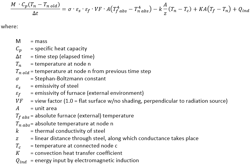
Dividing a cross-section of a steel billet into nodes, we can start by looking at the energy balance for each node:

All this equation is saying is that the change in the quantity of energy in a given node per unit time is equal to the sum of the energy flows into and out of the node. The quantity to the left is the accumulation terms while the quantities on the right side of the equation are terms for radiative heat transfer from the environment to the surface of the steel, conductive heat transfer between nodes within the steel, convective heat transfer between the external atmosphere and the steel, and inductive heat transfer into the steel.

Let’s start by breaking the mass in the accumulator term down as follows:

We continue by eliminating the convection and induction terms because they are comparatively small or nonexistent, and then by dividing all the remaining terms by the unit area:

Next we can expand terms:

Steal a first order dependent variable from the fourth order term:

Substituting back into the previous equation yields:

Gathering terms we get:

The coefficients for the T_n terms and the T_c terms on the left side of the equation fill the initialized coefficient matrix while the terms on the right side of the equation fill the initialized source matrix. There is one T term for each node. The radiation transfer terms drop out for any node that isn’t on the surface of the piece of steel being heated. The conduction terms drop out between any two nodes that aren’t internally connected.

This equation gets written for each node individually and then the system of equations gets solved. All of the T_n terms for the new time step end up in the source matrix at the end. Note that the temperatures are all represented in absolute degrees.

Posted in Tools and methods | Tagged matrix solution techniques, sim_presentation_series, thermodynamics | Leave a comment

Search for:
Recent Posts
Recent Comments
Categories
Meta
October 2026

M T W T F S S

1 2 3 4

5 6 7 8 9 10 11

12 13 14 15 16 17 18

19 20 21 22 23 24 25

26 27 28 29 30 31

« Sep

Recent Posts

Recent Comments

Categories

Meta