
Reproducing A Clever Animation Product, Part 28

In keeping with this week’s theme of researching backward compatibility of the various projects I’ve worked on over the past year I decided to figure out why parts of my fast animation framework weren’t updating as expected. The short answer is that IE 11 (and presumably 10 and 9 as well) simply does not process more than one parameter passed to a scale command in a style.transform assignment. I originally saw this happen in the debugger using the transform property directly. Changing the code to use msTransform (both when hard-coded and when switched after detection) didn’t change the behavior.

Here’s the relevant code running in the IE 11 debugger, as it appears just after having executed the statement at line 957. (transformPrefix has the value of “msTransform” in this case.)
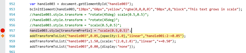
…and here is the value of the variable we have supposedly assigned:
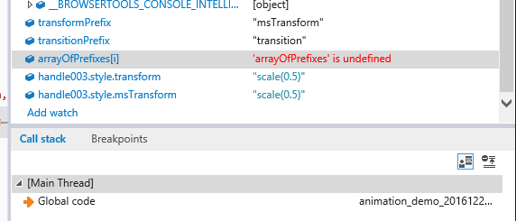
Doing the same thing in most other browsers results in the watch values taking on the expected result with both parameters. Although the Mozilla spec says that browsers should accept an optional second parameter, IE does not do so.

The solution, therefore,is to test to see if we’re running IE (9 or later?) and handle this scaling operation with only a single parameter as a special case. This means we cannot specify different scaling factors in the x- and y-directions but hey, it is what it is and it will do something. If we really, truly need to scale the axes independently then we can create a mechanism that uses the scaleX and scaleY commands separately.

I’ll implement the custom code tomorrow.

I used this code to detect which browser I was using and which prefixes I should use.

transformPrefix is the only value relevant in this code but I’ve included the others to demonstrate that they can be used. The code I lifted from an online example (from 2012) didn’t test for the typeof result coming back as an empty string; I had to add that when I got that result in the various debuggers when testing the value transform. That used to be first in the list of parameters to the GetVendorPrefix call but I moved it to the end to ensure I captured other possible results first.

Once the value of transformPrefix is set it can be used in a couple of different ways:

It turns out that just using transform property in most modern browsers will achieve the desired results. This must be the outcome of many years of standardization by the vendors.

Posted in Tools and methods | Tagged , , | Leave a comment

A Simple Discrete-Event Simulation: Part 64

As I’ve been developing and experimenting with JavaScript over the last year-plus I’ve been more interested in showing my experience in simulation, graphics, and analysis than I have been with cross-browser- or backward-compatibility. If it ran on my phone (iPhone 5s and now 7) and the most recent versions of Firefox and Chrome then I was good. I found a few calls in my fast animation framework project that are going to need to be enhanced to support certain browsers and I’m going to revisit those, but I found myself being particularly annoyed by the fact that my stuff was no longer displaying properly on my 3rd-generation iPad. That iPad runs iOS version 9.3.5, which is in theory the final update for that device.

iOS is currently up to version 10.2 for more modern devices and it runs everything nicely. I therefore ran my discrete-event simulation project code through Babel (using its default, built-in conversion page) to see what features from JavaScript 6 I might be using. This is a more recent version of the language that might not be supported by the iPad’s slightly older OS. I knew I was using default function parameters from the latest spec but wasn’t sure if I might be using anything else. I may discuss Babel’s quirks on a different day but for now I’ll note that it didn’t appear turn up anything else. I went through and changed all the declarations that used default parameters to more traditional forms, sent it to my server, and tried it out on the iPad.

It didn’t work.

The next step was to plug the iPad into my Mac and walk through the code in the remote debugger. Sure enough, I’d missed changing one instance of a default parameter. When I fixed that and uploaded it again it ran just fine on the older device. Here it is below.

A direct link to the standalone page is here.

I noticed that my 3rd-gen iPad renders the lower canvas element, that shows the 3D animation built using the Three.js framework, with a white background. I don’t think I explicitly set the color for that background, it just seems to default to black on newer devices so I didn’t think more about it. I’ll see about setting it explicitly to black going forward.

I also notice that the simulation and its animations run a lot slower on the older device. The iPad 3 was the first to incorporate the hi-res Retina Display but still used an older CPU so the device was considered to be a bit strained. Most of the work of running the simulation involves generating the graphics. I’ll eventually make it so the animations can be turned off independently under user control and also so the simulation itself can run at full speed without having to wait for calls to the animation loop. Those should run pretty quickly even on older devices, but as I’ve discussed previously, that is ultimately a question of the scope and scale of a simulation.

Posted in Simulation | Tagged , , | Leave a comment

A Simple Discrete-Event Simulation: Part 63

Today I finally implemented the first part of the reporting capability. So far the system keeps track of the total time spent trying to get through the major process areas and through the entire system as well. The entities are time stamped when they enter the system and also when they enter a new process area. The results are collected in time buckets (which have been set to 30 units in this example) whenever an entity leaves a process area or exits the entire system.

Determining when the entities enter and leave the entire system is straightforward but determining when they enter and leave each process area is more complex. What I did was create a componentGroup property for each component in the model. The various Process components, either singly or in groups, determine the process areas. The Queue components that feed each Process components or set of Process components are also given the same componentGroup label. Path components are not given labels and do not figure into this calculation (for now). Process components 1, 2, and 3, along with Queue components 0, 1, 2, and 3 were labeled as being part of the “Primary” group. Process components 10 and 11 and Queue component 10 were labeled as the “Secondary” group. A default group is created for the entire “System.” For the current iteration of the code I labeled all of the components by hand using a setComponentGroup method. It should be possible to only label the Process components and then have the system automatically identify the Queues that feed them but there are some complications that may arise with that. (I’ll add a note to the To Do list.)

When a Queue component or Process component receives an entity it checks to see if the entity’s componentGroup label is different than that of the component itself. If it is, then the entity’s componentGroup is given the value of the component and the entity is time stamped. Here’s where the fun begins: at this point the system updates a counter in the current interval bucket of the global stats data structure. In our current system this happens in Queue components 0 and 10. When the entity is forwarded from a Process component the remainder of the data is written to the global stats data structure. This involves incrementing a count, adding the elapsed residence time for the process area to an accumulator, checking to see if the residence time is a new highest or lowest value for the current interval, recording the new number of entities in the process area, and checking to see whether that value is a new high or low for the current interval.

A new stats timing component updates the bucket index at defined intervals (again, 30 time units for our example), and ensures that the global stats data structure is expanded to hold the next interval’s data. When the model run is complete the data is processed to output nice tables of results in the scrolling text area. It generates a table for each process area and each table includes a line for each time interval and a line for the totalized results for the run. Go ahead and run the model and see what results it generates. I’ve included an example output here.

A good bit of thought can go into what each of these results actually mean. For now, the residence time in the system and each process area is simply the total time the entity spent there. If we want to know how long an entity waited to be processed, however, that would be a different story. In that case we’d have to subtract the amount of time it takes to traverse the queues and links within a process area. If an entity passed straight through without delay then we’d say that the waiting time was zero, would we not? There are also counters for the number of entities in each area, but we may or may not want to count the ones that are actively being processed in a Process component. We’ll explore this going forward, and I’ll add still another To Do item.

This capability can be made a lot more complex. Statistics can be captured for different meta time periods (e.g. by day as well as by interval and for the run as a whole) or counts can be added for each component or group of like components (e.g., the number of entities using each entry or exit, the number processed in each “Primary” Process component or each “Secondary” process component). Resource use and availability can also be added when those features are added to the model. Graph and formatted print outputs can also be generated. The possibilities are almost endless, but this was a pretty fair start.

Posted in Simulation | Tagged , | Leave a comment

A Simple Discrete-Event Simulation: Part 62

Today I added the ability for the user to control how the display is updated. Two new buttons have been added to the button row between the 2D display and the 3D display. The second button from the right, labeled “Time” when the page is initialized, indicating that the animations will only be updated on a time interval determined by a new display control timer component. The base multiple is set to 0.5 so the model will process as many discrete-event items during each interval of that length, at which time it will update the appropriate displays. This is done once per screen refresh cycle. This makes the animation much easier to watch, and it also ensure that simulated time advances at a consistent rate. Clicking on that button will change the display to “Ops,” short for Operations, indicating that only one discrete-event item will be processed per screen refresh, and the displays will be updated in the manner we’ve seen up until now.

The rightmost button, labeled “x1” to start, governs the multiplier for the time interval. Clicking on it changes the display to “x2” and multiplies the default time interval for time-based updates by two. The multiplier applies to whatever the base time interval is. If the base interval is set to 0.25 time units then setting the multiplier to two will result in updates occurring every 0.5 time units. The multiplier value does not apply when the display is in “Ops” mode. In theory the multiplier could be set to any positive value above zero (including fractional values) but the demo uses one and two for simplicity.

Last but not least notice that changing the multiplier value takes effect after the next update is completed. This is because the next discrete-event item that triggers the display update has already been inserted into the future events queue using the old multiplier value.

Posted in Simulation | Tagged | Leave a comment

A Simple Discrete-Event Simulation: Part 61

If everything is right to this point then additional components and logic should be able to be added in any way desired. The complexity was increased by quite a lot and only turned up one minor code change. That’s a win in my book. I also compressed the 2D display components a little bit more.

What we have here is a system with three primary process points. Twenty percent of the entities processed are routed over to the secondary queue, which feeds two secondary processes. From there, twenty percent of the entities go to the secondary exit while most go to the primary exit. This might represent a manufacturing system with a primary inspection step. Items failing the inspection get sent to a secondary process to see if the issue can be fixed. If not, the item gets scrapped. If the model was of a simple land border crossing the secondary exit would represent a return to the country of origin. With just a few components we can model a wide variety of processes, but that won’t stop us from adding even more components to give us even more capabilities.

The simulation is taking longer and longer to run with increasing complexity, as we might expect. However, the framework currently redraws the scene after every individual event is processed and can only update sixty times per second. This is great for single-step debugging but a little painful to watch. What we’ll do, then, is change the framework to update the display in uniform increments of modeled time. That speeds things up a lot when a bunch of things are happening in rapid succession but slows things down when not much is happening. I will ultimately give the user complete control over how this update process is handled, including the ability to run the model with no animated display at all. At some point the various animations are only there to confirm that the model is working the way we want it to. The results it generates are entirely independent of the display.

Results? We’ll talk about how to generate those going forward as well.

Posted in Simulation | Tagged | Leave a comment

A Simple Discrete-Event Simulation: Part 60

Here the rendering output is piped through a transform that produces a stereoscopic display with slightly offset views. Make the element full screen then check it out using your favorite 3D goggles (Google Cardboard should do nicely).

Here’s a direct link if you can’t expand the frame to full screen in a mobile browser. Click here! Be sure the device is in landscape mode before activating the link.

Posted in Simulation | Tagged , , , | Leave a comment

A Simple Discrete-Event Simulation: Part 59

After attaching some new functionality, drawing the paths using the DisplayElements objects, defining 3D elements using the information already available, and learning some more about the Three.js framework and WebGL, we have a nice 3D display. There are many possible improvements but this illustrates the basic capability nicely.

Posted in Simulation | Tagged , , | Leave a comment

A Simple Discrete-Event Simulation: Part 58

Today I started experimenting with the Three.js framework that supports the creation of WebGL apps in most modern browsers. I started from the most basic example I saw demonstrated at a recent JavaScript Meetup in Baltimore. I then began to dig around to figure out how to add an modify things the way I wanted them. I first figured out how to display both the faces and the vertices of 3D shapes, and then I figured out how to make the camera fly around the correct axis to maintain the perspective I was going for. If x is left and right, y is up and down, and z is into the screen, then to make it look like you’re a helicopter flying around a landscape while always looking toward the same point you have to assume that the y-axis is the vertical about which you orbit (revolve) along or above the x-z plane. Now that I have that sorted out a lot of the rest of rendering the simulation in 3D should be fairly straightforward, if detailed and time-consuming.

Here’s the basic code so far.

I’m used to doing most of this sort of thing on my own by managing my own coordinates, transforms, perspecitives, and renderings, but I never fully studied hidden surface algorithms, shading, and so on. Learning this framework gives me a lot more leverage, and my existing experience helps me understand the whole thing easily enough.

Posted in Simulation | Tagged , , | Leave a comment

A Simple Discrete-Event Simulation: Part 57

Today I got a number of things done. I’ll describe them briefly but forego the code listings for today. Too much going on.

I created an external way to graphically represent the non-Path components. These work roughly the same way as the data display objects I’ve been using (and am still using for the Arrivals component, which doesn’t even have to be displayed) but take up much less space and display the entities that are within them. The entities in components are also colored differently depending on whether they have finished their process or traversed their queue. A bare minimum of queue information is provided, and this could probably be eliminated for the simple, one-element process component. This method of display should make things much more visually clear to the user.

The incoming and outgoing nodes are included in the representation of each component. This process will be extended to handle display of the Path components as well, for consistency.

The start and end coordinates of all Path components are now set automatically by referencing the incoming or outgoing node on the non-Path component to which they are attached. The start and end locations still have to be established manually where Path components are attached to each other in series. Still, this saves a lot of hassle for the designer. The code for this was added near then end of the verifyModel function.

This new representation allows more complex systems to be represented in less space. Eventually a lot of the labels and internal information can be squeezed out as well, to allow even more information to be displayed. The amount of information to display or not display should be as flexible and configurable as possible.

The original data display objects are still available. I plan to make them visible by user request to monitor more details than are shown in this newly streamlined version.

Posted in Simulation | Tagged | Leave a comment

A Simple Discrete-Event Simulation: Part 56

I the process of working off some of the TODO: items I have sprinkled through the code I ended up fleshing out the model verification function. It is called after everything is defined but before the model runs. I haven’t let a negative finding prevent the model from running — yet — since I currently have a working configuration. The function also ensures that certain settings are initialized.

Here’s the function itself. Explanations and supplementary listings follow.

The function starts out by verifying that all previous and next component links exists and are valid in a number of ways. Here’s an example of the most general formation. A customized version of the verifyLinks method was created for each component type. Component types that do not support one type of link or another (e.g., Exit components do not include forward connections) do not test those elements. It is possible that these methods can be even more standardized and modularized, and I may look into that at some point.

In general, the method ensures that the count of connections is not zero, that the list of connections does contain references to something, that the references are to objects, that the objects are (likely to be) components by testing for the presences of the componentType property, and that the connections are not to types of components that make no sense (e.g., Entry components cannot be connected to Exit components and vice versa).

The function continues by setting the value of the exclusive property for each Path component based the exclusive property of its terminating non-Path component. This assumes that the exclusive property of each non-Path component has already been set.

Here’s the getNextExclusive function I had to define in the Path component. I noticed that I do this pass-through thing frequently and should come up with a consistent naming convention for methods like this.

The verifyModel function then tests the nextComponentList links of every Entry component to ensure that all connected components are defined to be non-exclusive. Here’s the code for the A customized version of the verifyLinks method was created for each component type. method.

Finally, I moved the mechanism for assigning destination component indices for forward links to here.

Some of the methods return error codes, and these are placed in the scrolling text area. The messages include detailed notes about the components and connections that are incorrectly configured.

I have a comment in place to implement a mechanism to assign the desired distribution method based on the nature of the downstream connections.

I currently have the routing logic attached to the individual components, but there is also a need to ensure that certain combinations of destinations can be reached from the point of view of an entity moving through a system. Moreover, destinations may need to be identitied in an aggregate way, like a toll plaza containing many booths. I will implement a test mechanism to address that process at some point as well.

There are many more things that can be tested or automated in this or similar functions. However, this was a pretty good start.

Last but not least, and not related to this project, I was able to complete another class on Udemy over the weekend, this time about Sass and SCSS.

Posted in Simulation | Tagged | Leave a comment