
“It was smooth sailing” vs. “I hit every stinkin’ red light today!”
Think about all the factors that might affect how long it takes you to drive in to work every day. What are the factors that might affect your commute, bearing in mind that models can include both scheduled and unscheduled events?
- start time of your trip
- whether cars pull out in front of you
- presence of children (waiting for a school bus or playing street hockey)
- presence of animals (pets, deer, alligators)
- timing of traffic lights
- weather
- road conditions (rain, slush, snow, ice, hail, sand, potholes, stuff that fell out of a truck, shredded tires, collapsed berms
- light level and visibility
- presence of road construction
- occurrence of accidents
- condition of roadways
- condition of alternate routes
- mechanical condition of car
- your health
- your emotional state (did you have a fight with your significant other? do you have a big meeting?)
- weekend or holiday (you need to work on a banker’s holiday others may get)
- presence of school buses during the school year, or crossing guards for children walking to school
- availability of bus or rail alternatives (“The Red Line’s busted? Again?”)
- distance of trip (you might work at multiple offices or with different clients)
- timeliness of car pool companions
- need to stop for gas/coffee/breakfast/cleaning/groceries/children
- special events or parades (“What? The Indians finally won the Series?”)
- garbage trucks operating in residential areas
So how would you build such a simulation? Would you try to represent only the route of interest and apply all the data to that fixed route, or would you build a road network of an entire region to drive (possibly) more accurate conditions on the route of interest? (SimCity simulates an entire route network based on trips taken by the inhabitants in different buildings, and then animates moving items proportional to the level of traffic in each segment.)
Now let’s try to classify the above occurrences in a few ways.
- Randomly generated outcomes may include:
- event durations
- process outcomes
- routing choices
- event occurrences (e.g., failure, arrival; Poisson function)
- arrival characteristics (anything that affects outcomes)
- resource availability
- environmental conditions
- Random values may be obtained by applying methods singly and in combination, which can result in symmetrical or asymmetrical results:
- data collected from observations
- continuous vs. discrete function outputs
- single- and multi-dice combinations
- range-defined buckets
- piecewise linear curve fits
- statistical and empirical functions (the SLX programming language includes native functions for around 40 different statistical distributions)
- rule-based conditioning of results
Monte Carlo is a famous gambling destination in the Principality of Monaco. Gambling, of course, is all about random events in a known context. Knowing that context — and setting ultimate limits on the size of bets — is how the house maintains its advantage, but that’s a discussion for another day! When applied to simulation, the random context comes into play in two ways. First, the results of individual (discrete) events are randomized, so a range of results are generated as the simulation runs over multiple iterations. The random results are generated based on known distributions of possible outcomes. Sometimes these are made by guesstimating, but more often they are based on data collected from actual observations. (I’ll describe how that’s done, below.) The second way the random context comes into play is when multiple random events are incorporated into a single simulation so their results interact. If you think about it, it wouldn’t be very interesting to analyze a system based on a single random distribution, because the output distribution would be essentially the same as the input distribution. It’s really the interaction of numerous random events that make such analyses interesting.
First, let’s describe how we might collect the data from which we’ll build a random distribution. We’ll start by collecting a number of sample values using some form of the observation technique from the BABOK, ensuring that we capture a sufficient number of values.
What we do next depends on the type of data we’re working with. In the two classic cases we order the data and figure out how many occurrences of each kind of value occur. In both cases we start by arranging the data items in order. If we’re dealing with a limited number of specific values, examples of which could be the citizenship category of a person presenting themselves for inspection at a border crossing or the number number of separate deliveries it will take to fulfill an order, then we just count up the number of occurrences of each measured value. If we’re dealing with a continuous range of values that has a known upper and lower limit, with examples being process times or the total value of an order, then we must rearrange the data in order and break it into “buckets” across intervals chosen to capture the shape of the data accurately. Sometimes data is collected in raw form and then analyzed to see how it should be broken down, while in other cases a judgment is made about how the data should be categorized ahead of time.
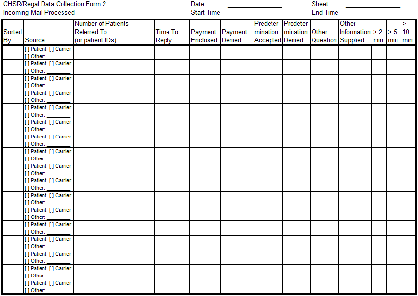
The data collection form below shows an example of how continuous data was pre-divided into buckets ahead of time. See the three rightmost columns for processing time. Note further that items that took less than two minutes to process could be indicated by not checking any of the boxes.
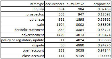
In the case where the decision of how to analyze data is made after it’s collected we’ll use the following procedures. If we identify a limited number of fixed categories or values we’ll simply count the number of occurrences of each. Then we’ll arrange them in some kind of order (if that makes sense) and determine the cumulative number of readings and determine the proportion of each result’s occurrence. A random number (from zero to one) can be generated against the cumulative distribution shown below, which determines the bucket and the related result.
Given data in a spreadsheet like this…
…the code could be initialized and run something like this:
|
1 2 3 4 5 6 7 8 9 10 11 12 13 14 15 16 17 18 19 20 21 22 23 24 25 26 27 28 29 30 31 32 33 34 35 36 37 38 39 40 41 42 43 44 45 46 47 48 49 50 51 52 53 54 55 56 57 58 59 60 61 62 63 64 |
//code in C++ //global values, or declared in a unit const char discreteLabelArray[10][14] = {"inquiry", "prospectus", "purchase", "sale", "statement", "advertisement", "update", "dispute", "open account", "close account" }; const int discreteRawDataArray[10] = {384,563,951,1104,382,1429,11,56,158,111}; float discreteCumulativeDistribution[10]; //initialize the working array against which the random numbers will be tested void initDiscreteCumulativeDistribution() { int i; float total; float discreteCumulativeArray[10]; total = 0.0; for(i=0; i<10; i++) { total += discreteRawDataArray[i]; discreteCumulativeArray[i] = total; } for (i=0; i<10; i++) { discreteCumulativeDistribution[i] = discreteCumulativeArray[i] / total; } } //generate random number and identify bucket, then return index int generateDiscreteIndex() { int i; float dieroll,normalized; //this language implementation generates randoms from zero to the specified integer dieroll = random(1000000); //...which must be converted to a floating point between zero and one normalized = dieroll / 1000000.0; //test against the normalized array, identify bucket i = 0; while (normalized > discreteCumulativeDistribution[i]) { i++; } //return the index directly return i; } //calls of above functions where appropriate //initialization initDiscreteCumulativeDistribution(); //generate the live index int index = generateDiscreteIndex(); //get the associated string, if needed char resultLabel[14]; strcpy(resultLabel,discreteLabelArray[index]); |
There are always things that could be changed or improved. For example, the data could be sorted in order from most likely to least likely to occur, which would minimize the execution time as the function would generally loop through fewer possibilities. Alternatively, the code could be changed so some kind of binary search is used to find the correct bucket. This would make the function run times highly consistent at the cost of making the code more complex and difficult to read.
This is pretty straightforward and the same methods could be used in almost any programming language. That said, some languages have specialized features to handle these sorts of operations. Here’s how the same random function declaration would look in GPSS/H, which is something of an odd beast of a language that looks a little bit like assembly in its formatting (though not for its function declarations). GPSS/H is so unusual, in fact, that the syntax highlighter here doesn’t recognize that language and color it consistently.
|
1 2 3 |
12345 FUNCTION RN1,D0010 COMMENTS COMMENTS COMMENTS 0.074580,01/0.183920,02/0.368620,03/0.583030,04/0.657210,05/0.934740,06/0.936880,07/ 0.947760,08/0.978440,09/0.999999,10 |
In this case the 12345 is an example of the function index, the handle by which the function is called. RN1 indicates that the random function iterates a die roll of 0.0-0.999999 between the first values in each pair and, when the correct bucket is found, returns the second value. D0010 indicates that the array has ten elements. The defining values are given as a series of x,y value pairs separated by slashes. The first number of each pair is the independent value while the second is the dependent value.
The language defines five different types of functions. Some function types limit the output values to the minimum or maximum if the input is outside the defined range. I’m not doing that in my example functions because I’ve limited the possible input values.
So that’s the simple case. Continuous functions do mostly the same thing but also perform a linear interpolation between the endpoints of each bucket’s dependent value. Let’s look at the following data set and work through how we might condition the information for use.
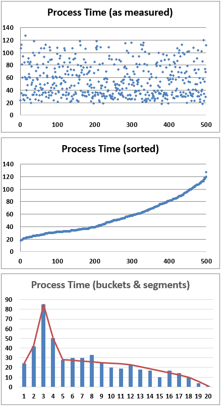
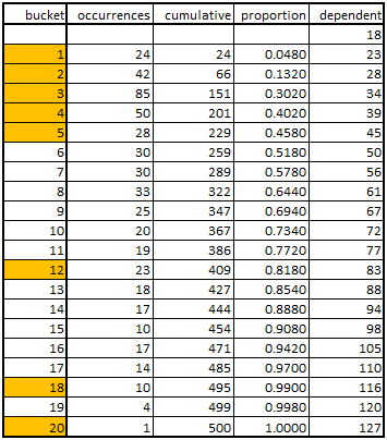
In this case we just divide the range of observed results (18-127 seconds) by 20 buckets an see how many results fall into each range. We then do the cumulations and proportions like before, though we need 21 values so we have upper and lower bounds for all 20 buckets for the interpolation operation. If longer sections of the results curve appear to be linear then we can omit some of the values in the actual code implementation. If we do this then we want to shape a piecewise linear curve fit to the data. The red line graph superimposed on the bar chart above shows that the fit including only the items highlighted in orange in the table is fairly accurate across items 5 through 12, 12 through 18, and 18 through 20.
The working part of the C++ code would look like this:
|
1 2 3 4 5 6 7 8 9 10 11 12 13 14 15 16 17 18 19 20 21 22 23 24 25 26 27 28 29 30 31 32 33 34 35 36 37 38 39 40 41 42 43 44 45 46 47 48 49 50 51 52 53 54 55 56 57 58 59 60 |
//code in C++ //global values, or declared in a unit const int continuousRawDataArray[8] = {24,42,85,50,28,180,86,5}; float continuousCumulativeDistribution[8]; float continuousDependentValueArray[9] = {18,23,28,34,39,45,83,117,127}; //initialize the working array against which the random numbers will be tested void initContinuousCumulativeDistribution() { int i; float total; float continuousCumulativeArray[8]; total = 0.0; for(i=0; i<8; i++) { total += continuousRawDataArray[i]; continuousCumulativeArray[i] = total; } for (i=0; i<8; i++) { continuousCumulativeDistribution[i] = continuousCumulativeArray[i] / total; } } //generate random number and identify bucket, then return index float generateContinuousResult() { int i; float dieroll,normalized,result,a,b,c,d; //this language implementation generates randoms from zero to the specified integer dieroll = random(1000000); //...which must be converted to a floating point between zero and one normalized = dieroll / 1000000.0; //test against the normalized array, identify bucket i = 0; while (normalized > continuousCumulativeDistribution[i]) { i++; } //interpolate piecewise linear curve fit if (i > 0) { a = continuousCumulativeDistribution[i-1]; } else { a = 0.0; } b = continuousCumulativeDistribution[i]; result = (normalized - a) / (b - a); c = continuousDependentValueArray[i]; d = continuousDependentValueArray[i+1]; result = c + result * (d - c); return result; } //calls of above functions where appropriate //initialization initContinuousCumulativeDistribution(); //generate the live result float result = generateContinuousResult(); |
Looking at the results of a system simulated in this way you can get a range of answers. Sometimes you get a smooth curve that might be bell-shaped and skewed left. This would indicate that much of the time your commute duration fell in a typical window but was occasionally a little shorter but sometimes longer, and sometimes by a lot. Sometimes the results can be discontinuous, which means you sometimes get a cluster of really good or really bad overall results if things stack up just right. Some types of models are so granular that the variations kind of cancel each other out, and thus we didn’t need to run many iterations. This seemed to be the case with the detailed traffic simulations we built and ran for border crossings. In other cases, like in the more complicated aircraft support logistics scenarios we analyzed, the results could be a lot more variable. This meant we had to run more iterations to be sure we were generating a representative output set.
Interestingly, exceptionally good and exceptionally poor systemic results can be driven by the exact same data for the individual events. It’s just how things stack up from run to run that makes a given iteration good or bad. If you are collecting data during a day when an exceptionally good or bad result was obtained in the real world, the granular information obtained should still give you the more common results in the majority of cases. This is a very subtle thing that took me a while to understand. And, as I’ve explained elsewhere, there are a lot of complicated things a practitioner needs to understand to be able to do this work well. The teams I worked on had a lot of highly experienced programmers and analysts and we had some royal battles over what things meant and how things should have been done. In the end I think we ended up with a better understanding and some really solid tools and results.