
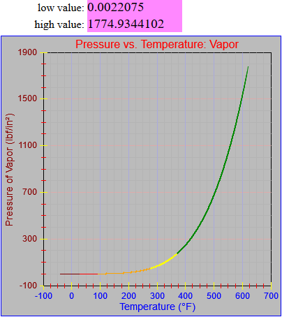
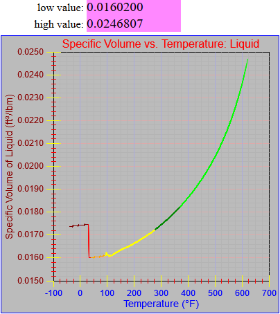
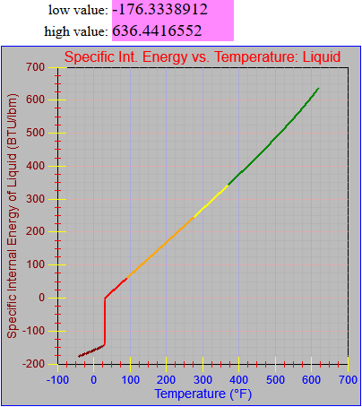
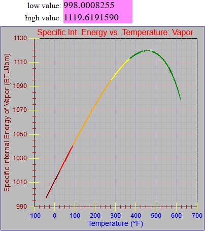
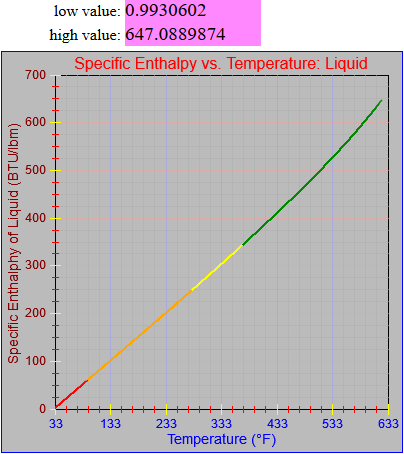
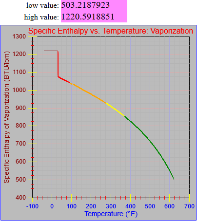
Here are plots of the standard thermodynamic values for saturated water, all as a function of temperature. Tomorrow I’ll plot them all out as a function of pressure.
I extended the range of each function below 32 degrees Fahrenheit to address conditions that occurred in a model I build earlier in my career. For those lower temperatures the water is not saturated but exists either in a subcooled state in the liquid phase of the superheated state in the vapor phase. Many of these function exhibit a discontinuity at 32 degrees. I apparently used data from a different set of tables which I’ll try to identify going forward, particularly as I work through the process of recreating the curve fits I did and correcting those that seem obviously in error. I’ll be working through that process next week.
I also believe that I’ve figured out why the plotted lines are so thick and why they often include small bulges that make the plot look like it’s chattering up and down unexpectedly. The effect appears to be caused by drawing lines with the lineCap mode set to “square,” which adds nearly a full pixel to either end of each plotted line segment. Since the curves are drawn at one-pixel intervals along the x-axis any pixel changes along the y-axis should result in extra thick lines or lone pixels above or below the plotted line. Tomorrow I will try producing the graphs with the lineCap mode set to “butt.”
There are clearly a few segments that look awry on these graphs, and they are usually at the lower end of the temperature scale, above 32 and less than 100 degrees. Re-fitting the curves will require me to implement a few of the features on my to-do list for the graph project, as well as demonstrating how the curve function were created in the first place.

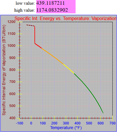
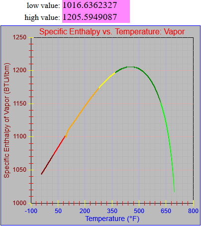
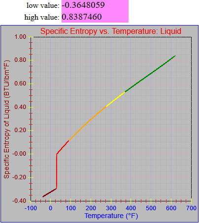
Finally, here is an example of one of the thermodynamic functions. It is composed of individual curve fits across a limited range or temperatures, and the value for a global variable called graphCycle is set to an index based on which of the fits are used. That index is used to select the color in which that section of the function’s output curve is to be drawn. If the input value is out of the range covered by the function the value for graphCycle is set to a different constant indicating that the input value is lower or higher than the active range. In those cases no line segments are added to the graph.
|
1 2 3 4 5 6 7 8 9 10 11 12 13 14 15 16 17 18 19 20 21 22 23 24 25 26 27 28 29 30 31 32 33 34 35 36 37 38 39 40 41 42 43 44 45 46 47 48 49 50 51 52 53 54 55 56 57 58 59 60 61 |
function TFind_P(T) { var temp = 0.0; if (T < -40.0) { graphCycle = graphCycleBottom0; temp = 0.0; } else if (T < 32.018) { graphCycle = 1; T = T + 4.00000000000000E+0001 + 2; temp = -5.82750190795537E-0004; temp += ( 3.10138202245116E-0004 * T); temp += (-9.96845835382852E-0006 * T * T); temp += ( 2.93452465077397E-0007 * T * T * T); temp += 1.90000000000000E-0003; } else if (T <= 95) { graphCycle = 2; temp = 1.02291643993728E-0001 * T; temp += (-1.56461430882940E+0001 / T); temp += (-7.77500161911500E-0001 * Math.sqrt(T)); temp += (-5.68581901662451E-0001 * Math.log(T)); temp += (-5.57135053654371E-0004 * T * T); temp += ( 2.68643222990479E-0006 * T * T * T); // temp += 4.06678025391659E+0000 + 8.86600000000000E-0002;} temp += 4.15544025391659E+0000; } else if (T <= 281.03) { graphCycle = 3; temp = 3.92079417112400E+0001 * T; temp += ( 4.01213788918853E+0004 / T); temp += (-1.28706905409880E+0003 * Math.sqrt(T)); temp += ( 3.50936122348532E+0003 * Math.log(T)); temp += (-3.40581930733492E-0002 * T * T); temp += ( 3.01211718278793E-0005 * T * T * T); temp += -7.30111133292317E+0003; temp += 0.00000000000000E+0000; } else if (T <= 373.13) { graphCycle = 4; temp = -4.46073180369288E+0003 * T; temp += (-2.91401612241211E+0007 / T); temp += ( 2.35876174171448E+0005 * Math.sqrt(T)); temp += (-1.02466834830570E+0006 * Math.log(T)); temp += ( 1.41416476892482E+0000 * T * T); temp += (-3.85708716196032E-0004 * T * T * T); temp += 3.07749988717651E+0006; temp += 5.00000000000000E+0001; } else if (T <= 621.21) { graphCycle = 5; temp = 6.08822615030408E+0003 * T; temp += ( 6.96757841217041E+0007 / T); temp += (-3.68132442183495E+0005 * Math.sqrt(T)); temp += ( 1.83794467631912E+0006 * Math.log(T)); temp += (-1.51896496594964E+0000 * T * T); temp += ( 3.61841945230257E-0004 * T * T * T); temp += -6.03886787577057E+0006; temp += 1.80000000000000E+0002; } else { graphCycle = graphCycleTop0; temp = 0.0; } return temp; } |