
While continuing the process of turning the JavaScript graph widget into an object I found I needed to create labels of various kinds, which you see added in the examples below. I also wanted to test out some more of the thermodynamic functions I wrote when I was doing power plant simulations. The graphs I generated for specific enthalpy of saturated fluid (hf), specific enthalpy of vaporization (hfg), and specific enthalpy of saturated vapor (hg) are shown below.
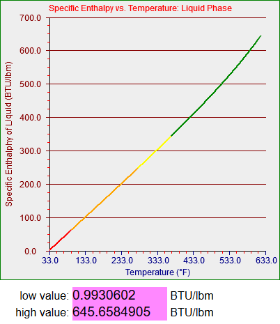
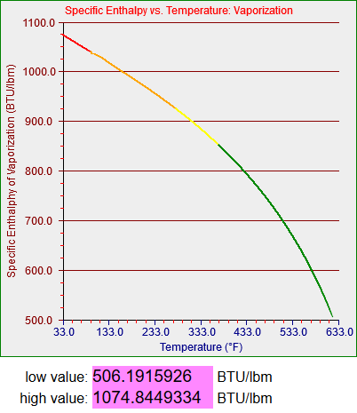
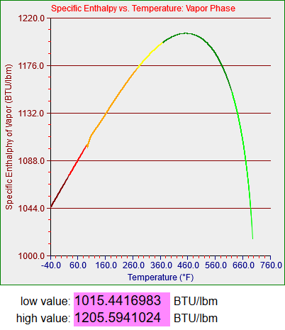
These graphs represent represent the thermal energy contained per unit mass of saturated water in its liquid and gaseous states and the amount of energy it takes to transition between the two. If you’re not a thermodynamics geek its not all that important. What you need to know is that water is used in power plants (and a lot of other applications) and you have to know how it acts in order to a) design the plant and b) model said plant, as we did for the training simulators.
Strictly speaking the saturation curves for water are only defined between 32.018 degrees Fahrenheit (0.0866 psi) and 705.44 degrees Fahrenheit (which occurs at 3204 psi). Since my models didn’t have to deal with temperatures higher than about 560 degrees Fahrenheit (around 1100 psi, the operating pressure in a boiling water reactor or BWR) my steam tables only had to cover up to somewhere in the low 600s. One of my models did have to deal with very low temperatures, however, which story I’ll get to.
The two graphs above are plotted from 33 degrees to 633 degrees and the graphing function is in this case designed not to graph the segments that make discontinuous jumps to zero. (I’ll have to deal with that when I generalize the functions that may include values both above and below zero.) The bottom graph, for vapor, however, is plotted from -40 to almost 700 degrees. The upper section was generated as a normal curvefit but the lower section appears to be generated by a linear function I developed. As I mentioned above any water vapor that exists in a region below 32 degrees will be superheated and not saturated. I think what I must have done was to use a different source for the properties of superheated vapor and simply extend the function and graph as shown. I do not actually remember what I did back then and I don’t have time to figure it out now. However, the section of the model that inspired me to do this work needed to represent vapor at temperatures somewhat below 32 degrees, and the functions I wrote seemed to work smoothly enough.
You can see from the two graphs below that I also extended the functions for enthalpy of fluid and enthalpy of vaporization down to -40 degrees as well. In these cases I’m not sure what the point was or how I generated the numbers. It looks like I assumed a constant heat of vaporization and generated the liquid curve by subtracting it from the vapor curve. I’d have to look at my notes to see what I was thinking, but I’m pretty sure any vapor that remained in the colder parts of the model was never allowed to condense into a liquid. At that point it should more or less have been treated as a contaminant in the air mixture that was being processed in the system I was simulating.
If nothing else, remember to take good notes. You may find yourself revisiting some very old code and scratching your head a lot (or wondering what you were drinking…). That said, I had developed a consistent way of representing what happened in the various model nodes of a system that contained high-pressure steam with a bit of air and dissociated hydrogen and oxygen at one end and cold, low-pressure air with traces of water vapor at the other, so I’m sure I developed the functions for completeness and consistency. It was a very, very challenging exercise, particularly for a modeler with as little experience as I had at he time. As I have described elsewhere I developed an entire continuous simulation framework so I could do my own testing and development. I had to learn a lot, and I had to do it quickly. Fortunately I had my own computer, the latest copies of Borland’s Pascal products, several books of steam tables, and no fear.
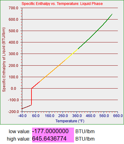
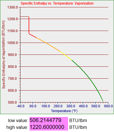
A couple of final notes are these. I mentioned that the graphs, which plot by sections, are set up to not draw discontinuities to zero, but they do draw internal discontinuities, as you can see in the two plots above. The numbers below each plot are widgets I added to the web page in question to record the range of non-zero y-values I generated for each function. I used those to help me identify the values to use on the y-axis. The more I work with these functions and the more I look at things I’ve done previously, the bigger this project gets.
Fortunately it’s fun!