
There are a large class of analogous engineering problems that may be addressed with a particular mathematical solution. Fluid systems where volumes containing fluid are connected by fluid flows, mechanical systems where masses are connected by springs and dashpots (which you can think of shock absorbers), electrical systems with nodes having voltage levels that are connected by currents, and thermal systems where nodes containing energy are connected by energy flows are all analyzed and solved in similar ways. The change in any quantity at a node is a function of the flows into and out of the node, the quantities stored in the node, the extent of the node, and the behavioral properties of the node. The specific equations may differ; current flow is a function of voltage differential over electrical resistance while fluid flow is a function of the square root of the pressure differential over the fluid flow resistance.
Let’s take a look at a simple fluid system.
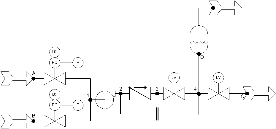
This system has four internal nodes, a pump, a collection of valves, an orifice plate, and connections to external systems. The tank, which contains a liquid section and a gaseous section, might be part of the system as it is logically defined, but it may or may not be considered part of the system that is included in a particular mathematical solution. In this case we’ll consider the bottom of the tank to be an external node.
To keep things really, really simple for today lets skip to a series of equations written int terms of the pressure at each node. There are several possible components to each coefficient. There can be what I’ll call an accumulation term, which has to do with each node, a resistance or conductance term which has to do with the connections between nodes, external driver terms which have to do with influences from outside systems, and internal modification terms which describe how things can change within the system. I’ll break this down in detail in the not-to-distant future.
A1P1 + B1P2 + C1P3 + D1P4 = E1dP/dt + F1
A2P1 + B2P2 + C2P3 + D2P4 = E2dP/dt + F2
A3P1 + B3P2 + C3P3 + D3P4 = E3dP/dt + F3
A4P1 + B4P2 + C4P3 + D4P4 = E4dP/dt + F4
The coefficients A through F may be different in each equation and may be composed of different values. If there is no connection between two nodes, then the coefficients describing connections between them will be zero. Nodes are always connected to themselves, so the diagonal terms in the coefficient matrix (elements 1,1, 2,2, 3,3, and 4,4) will always have values. The accumulation term will be written in the form of (accumulation term)(Pnew – Pold)/(increment of time) = (sum of flow effects) + (sum of internal effects). If we express the values and coefficients in matrix form we get the following:
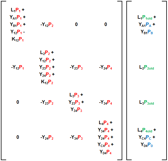
Here we see that the diagonal terms have an accumulation term, flow terms (some of which are driven by external connections), and in some cases internal effects (nodes 1 and 2 which represent the intake and discharge of a centrifugal pump). The off-diagonal nodes only have information about flow terms between connected nodes. Note that node 1 is not connected to node 3 or 4, so those terms are zero, while node 2 is connected to nodes 3 and 4, so those terms are non-zero. The results matrix has the old half of the accumulation term and, if appropriate, driver terms related to external connections.
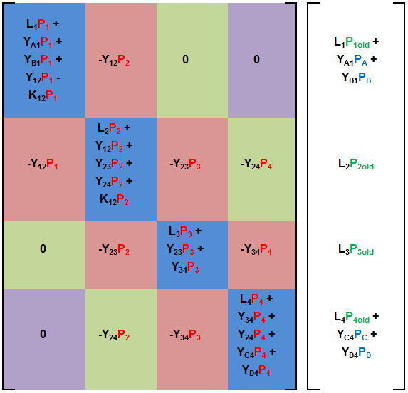
So, do we see anything special about this matrix? You might notice that the coefficients on opposite sides of the diagonal are the same. When this is true the matrix is said to be symmetric. This is nice because methods have been developed to solve symmetric matrix problems more efficiently than general matrix problems. It’s hard to see in this case but another thing you might notice is that a lot of the elements in the off-diagonal corners are filled with zeros. If those zeros make up nice, triangular patterns the matrix is said to be banded, and more efficient solutions have been developed for those cases as well. I’ve illustrated the banding in the figure below.
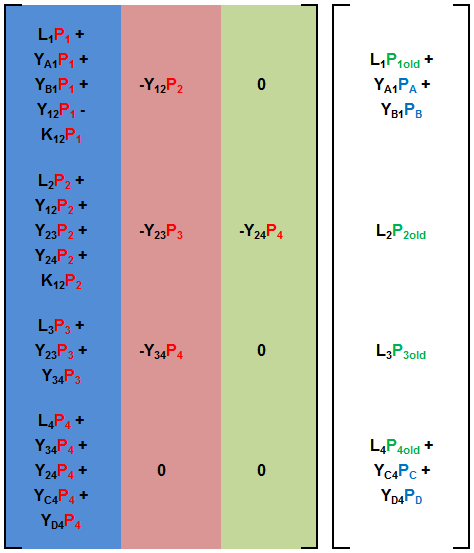
If a matrix is both symmetric and banded we can use even more efficient algorithms, if we rearrange the matrices as shown in the figure below.
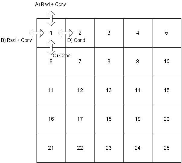
Let’s walk through this again with a larger system. Let’s say I want to model the flow of heat through a cross-section of material I’m trying to heat up. Each node has an area, an accumulated amount of energy, energy flowing to and from connected nodes (by conduction), and energy flowing to and from the external environment (by radiation and convection).
All of the energy flows are driven by temperature differentials (and other things), so we can write a series of equations for each node in terms of its temperature. The figure below shows a streamlined form of the equations without node or coefficient subscripts. The accumulation terms are represented by the coefficient A, external flows by E, and transport flows by T. I used X as the variable to be solved for, which in this case is temperature. The symmetry and banding are both very visible in this matrix:
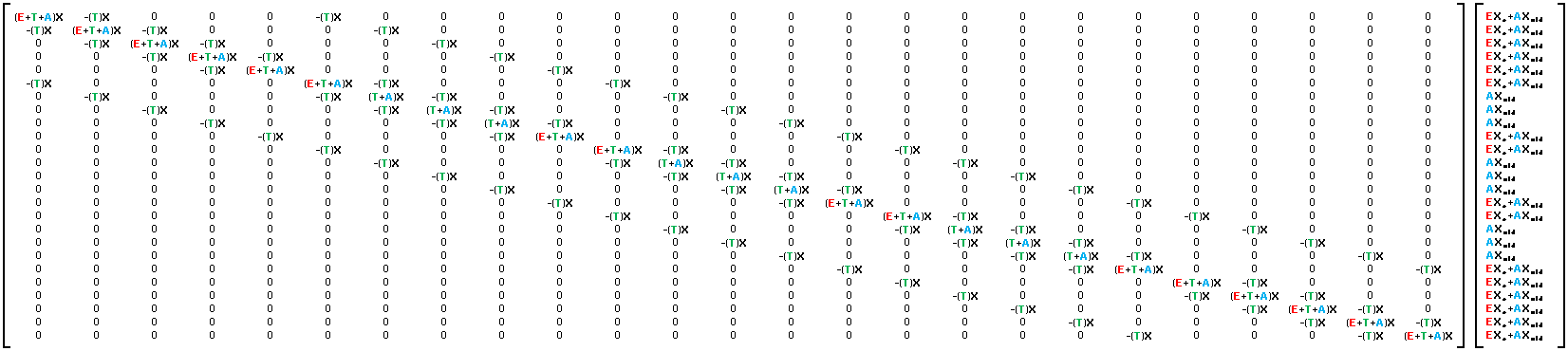
In this case we have accumulation and transfer terms in every entry on the main diagonal, as well as external driver terms for the surface nodes. The solution matrix has accumulation terms for each node and external driver terms for each surface node. Some of the surface nodes are missing transfer terms.
If we rearrange to get rid of the superfluous information we end up with the following:
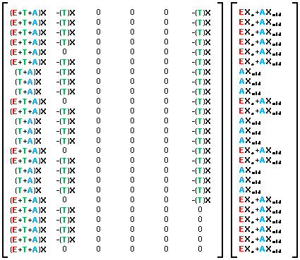
That, as I’ve discussed, looks like it could be solved much more quickly than the original matrix, doesn’t it?
The banding is very clear in this example, and it’s also clear that the configuration of nodes ensures that we have the narrowest bands possible. I proved this to myself once by calculating the narrowest possible band for every permutation of node order. This may not be a very important insight for such a regular and predictable configuration, but for unpredictable and irregular configurations the exercise is definitely worthwhile. You can name the nodes in any order you’d like, but you want to drop them into the matrix in the order that will yield the narrowest bands and the most efficient solution. This was done for the simulators built at Westinghouse. The Interactive Model Builder tool they created would do this automatically, and engineers who understood the technique applied it to their own models. I know I did for the model I wrote for the Offgas system.
I’ve described previously that there are ways to adjust the code to make even this efficient solution technique run faster. I’ll describe that in detail tomorrow.