Model-Predictive Industrial Control Systems
I combined everything I had learned about numerical techniques, programming, simulation, and computer graphics, added in some new knowledge about communicating between processes, and spent a number of fruitful years building model-predictive, supervisory control systems. A model-predictive simulation is used for control applications by doing the simulating the system into some future state using the current control settings. If the results do not match the target state the differences can be used to adjust the control settings.
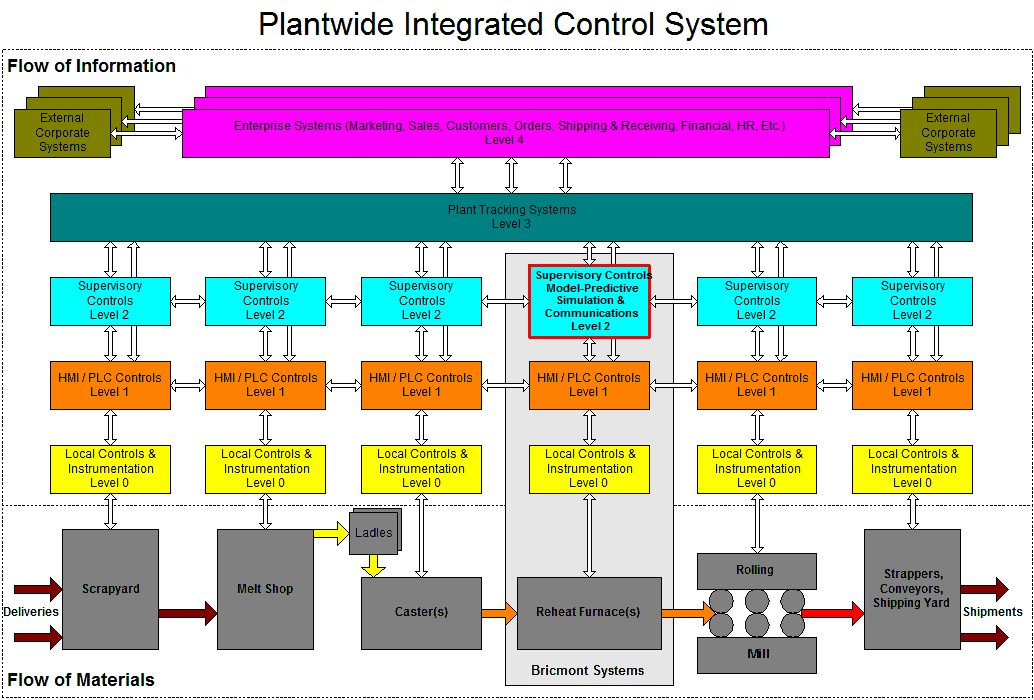
The low-level controls were based on PLCs, local hardware control loops, and an HMI package (e.g., Wonderware) running on one or more PCs. That, collectively, was the Level 1 system. It controlled the movement of the workpieces, controlled the fuel and air valves to manage combustion, controlled exhaust fans and dampers, handled safety interlocks, and displayed the status of everything in detail. I worked on the Level 2 system of supervisory controls. Its purpose was to read information from the Level 1 system about temperatures in the furnace, the types and locations of steel being heated, the current zone temperature setpoints, and the desired output temperatures of the steel. It would then use this information to update the temperature through some cross-section of the workpieces, which came in many geometries. This was necessary because the temperature inside the steel cannot be measured and the system had to ensure each piece was heated all the way through. That could only be done using a real-time simulation. The information from the Level 1 system, plus information from upstream Level 1 and Level 2 systems (from casters or a mill yard), and sometimes information from a plantwide Level 3 tracking system (see figure at the bottom of this page), would give the level 2 system all it needed to update current temperatures, calculate discharge average and differential temperatures, and changes to the zone setpoints. Depending on the installation, it would either display details about the temperature profiles of the workpieces directly, or it would relay the requested information back down to the Level 1 system, along with the control setpoints.
I did the model and control programs for DEC-based systems, which did not have their own GUI (they had text-based terminals you could use to monitor the status of the system), while a colleague set up those systems and wrote the low-level communication and monitoring programs. DEC VAX and Alpha machines were used in all the tunnel furnace applications but only one walking beam furnace early in my tenure with Bricmont (now owned by Andritz). I soon moved the company to PC-based control systems for all other types of furnaces. They were cheaper while being just as fast and almost as robust, and I could use Borland development tools (Delphi briefly and then C++ Builder versions 1 through 4), which were themselves inexpensive and gave me the opportunity to develop much more informative graphical displays and control interfaces. For those systems, however, I had to write every single line of code, handle every communication, and manage all the archiving and retrieval. Some of those systems totaled up to 50,000 lines between code, header, and screen definition files but I had a blast writing them. I was probably never more productive.
Stunningly, I was able to find the AT&T commercial from 1994 that inspired the 3D graphics I created to visualize the heating of the steel along its length and through its thickness.
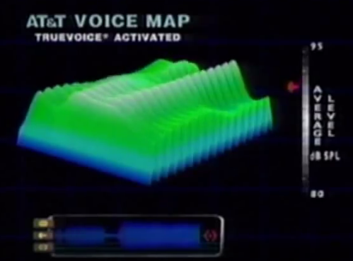
I added the isometric projection, coloration, and animation to make the idea my own. My colleagues and managers always made it a point to bring visitors by my desk after that, including the ones who ended up buying the company!
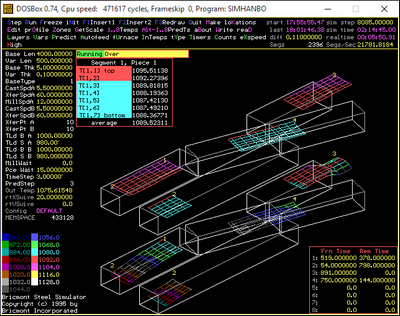
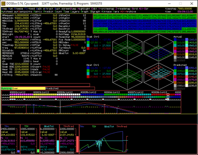
I extended the simulation test bed I'd created previously as I built my first reheat simulations. We ended up delivering these tools to more than one customer to help them work out control strategies and do a bit of light operations research. The image above shows a two-line tunnel furnace with swiveling transfer sections. The lower display shows the current temperature profile and location of each slab while the upper display shows the predicted discharge profile of the same slabs. The left-hand line in each case is line A, which discharges slabs to the rolling mill. In the lower display the top and bottom surfaces are cooling as the slab exits the furnace on the way to the first mill stand. The video below shows a two-line tunnel furnace with shuttles. Calculation and display of predicted temperatures was turned off so the animation would run more quickly.
The animations were cool enough, but what made the whole thing work was actually the matrix calculation methods I had learned at Westinghouse, especially when it came to extreme loop unrolling. I was amazed to find that I could not only calculate the updated temperature of every section of every slab in two furnaces, I could do so while simulating their movement out of the furnace, allowing calculation of their final average and differential temperatures at discharge -- all in under three seconds! That allowed me to control for output temperature using information from every piece in the furnace in real-time.
The tunnel furnace models ran every three or four seconds because they only required 1D calculations through the thickness of each slab, repeated along the center line from head to tail along the length of each slab. Pusher furnaces could often be modeled using a single, 1D calculation for each piece because their sides abutted each other and net heat transfer from side to side was negligible. The cycle times in those cases might have been ten seconds due to the number of pieces in the furnace and their longer residence times. Other pusher furnaces, along with all walking beam and walking hearth furnaces required 2D models of 49 to 127 nodes and took a lot longer to run. They required cycle times of 30-40 seconds.
I implemented systems like this in several languages (Pascal/Delphi, FORTRAN, C, and C++) on PCs and DEC VAX and Alpha machines. These systems all included multiple processes connected via shared memory. The processes exchanged data with other systems, performed temperature and control calculations, generated alarms, and archived, retrieved, and displayed historical data. Here's how the architecture for the Level 2 systems worked:
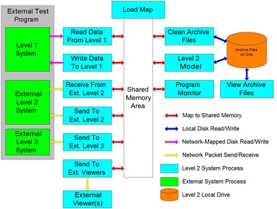
And here's how the Level 2 system fit in to the plant-wide system: